Vybrané partie z dátových štruktúr
2-INF-237, LS 2016/17
Táto stránka sa týka školského roku 2016/17. Od školského roku 2017/18 predmet vyučuje Jakub Kováč, stránku predmetu je https://kubokovac.eu/ds/
Poradie tém, poznámky, prezentácie:
Úvodné informácie
- Niektoré prednášky budú v angličtine, domácu úlohu, prezentáciu a skúšku však môžete robiť aj po slovensky.
Základné údaje
Rozvrh
- Uto 9:50-11:20 M-VIII
- Str 15:40-17:10 M-II
Vyučujúca
Ciele predmetu
- Oboznámime sa s dátovými štruktúrami nepreberanými na základných
bakalárskych predmetoch a s metódami ich analýzy. Zhrnieme tiež základné
algoritmy na vyhľadávanie vzorky (slova) v texte.
- Použitie a prehĺbenie znalostí z predchádzajúcich predmetov
týkajúcich sa tvorby a analýzy efektívnych algoritmov a dátových
štruktúr.
- Získavanie skúseností v práci s odbornou literatúrou, navrhovaní a vyhodnocovaní výpočtových experimentov.
Literatúra
- Dan Gusfield (1997) Algorithms on Strings, Trees and Sequences: Computer Science and Computational Biology. Cambridge University Press. Prezenčne v knižnici so signatúrou I-INF-G-8.
- Obsahuje časť učiva o sufixových poliach a stromoch
- Cormen, Thomas H., Charles E. Leiserson, Ronald L. Rivest, and
Clifford Stein. Introduction to Algorithms. MIT Press 2001. Prezenčne v
knižnici so signatúrou D-INF-C-1.
- Obsahuje napríklad amortizovanú analýzu
- Peter Brass. Advanced Data Structures. Cambridge University Press 2008. Prezenčne v knižnici so signatúrou I-INF-B-67
- Poznámky z predmetu Vyhľadávanie v texte [1]
- Obsahujú časti súvisiace s textom (vyhľadávanie kľúčových slov,
sufixové polia a stromy, LCA a RMQ, BWT, KMP, editačné vzdialenosť), ale
sú zčasti písané študentami a nedokončené
- Gnarley trees Stránka Kuka Kováča a jeho študentov s vizualizáciou dátových štruktúr
- MIT predmet Advanced Data Structures vyučovaný Erikom Demainom
- Ďalšiu literatúru uvedieme k jednotlivým témam
Prezentácia
Cieľom prezentácie je precvičiť si prácu s odbornou literatúrou a
oboznámiť sa s ďalšími výsledkami v oblasti dátových štruktúr. Každý
študent si zvolí a podrobne naštuduje jeden odborný článok (z odbornej
konferencie alebo časopisu) z tejto oblasti a ten odprezentuje
spolužiakom na prednáške koncom semestra. Každý študent si musí zvoliť
iný článok.
Termíny
- Výber článku na prezentáciu do pondelka 24.4. v systéme Moodle.
Každý článok môže prezentovať iba jeden študent, takže odovzdajte svoj
výber radšej skôr. Kto si článok do uvedeného termínu nevyberie, bude mu
nejaký priradený vyučujúcou.
- Prezentácie na prednáškach v posledných týždňoch semestra
- Prezentáciu vo formáte pdf odovzdať prostredníctvom Moodlu najneskôr 1 hodinu pred prednáškou, na ktorej máte prezentovať.
Rozvrh prezentácií
Rady k prezentácii
- Na prezentáciu budete mať 15 minút (plus diskusia), pričom tento
limit bude striktne dodržiavaný. Nechystajte si teda priveľa materiálu,
rátajte aspoň 1,5 minúty na slajd.
- K dispozícii bude dátový projektor a notebook, na ktorom bude
nahraná vaša odovzdaná prezentácia. Môžete si priniesť aj vlastný
počítač. Môžete použiť tabuľu, ale s mierou, lebo vysvetľovanie pri
tabuli ide pomalšie.
- Hlavným cieľom je porozprávať niečo zaujímavé z vášho článku vo
forme prístupnej vašim spolužiakom (ktorí chodili na tento predmet,
nepamätajú si však každý detail z každej prednášky). Nemusíte pokryť
celý obsah článku a nemusíte použiť rovnaké poradie, označenie alebo
príklady, ako autori článku.
- Nedávajte do prezentácie veľa textu, použite dostatočne veľký font a
dobre viditeľné farby (podobné farby, napr. žltá na bielej, nemusia byť
na projektore vôbec viditeľné).
- Použite čo najmenej definícií a označenia. Pojmy, algoritmy a
dôkazy radšej ilustrujte na obrázku alebo príklade, než zložitým textom.
Typická osnova prezentácie (podľa potreby ju však možete meniť):
- Úvod: aký problém autori študujú, prečo je dôležitý alebo
zaujímavý? Má nejaký vzťah k učivu z prednášok, prípradne k iným
predmetom?
- Prehľad výsledkov: V čom je presne prínos autorov oproti
predchádzajúcim prácam? Nemusíte robiť rozsiahly prehľad
predchádzajúcich prác, len uveďte, čo je v článku nové. Malo by to byť
jasné najmä z úvodu a záveru článku.
- Jadro: Vysvetlite nejaký kúsok zo samotného obsahu článku (časť
algoritmu alebo dôkazu, niektoré výsledky z testovania na dátach a pod.)
- Záver: zhrnutie prezentácie, váš názor (čo sa Vám na článku páčilo alebo nepáčilo)
Typy vhodných článkov
- Články o dátových štruktúrach alebo ich variantoch, ktoré neboli/nebudú pokryté na prednáške
- Články empiricky porovnávajúce dátové štruktúry na reálnych dátach
alebo popisujúce použitie týchto algoritmov v reálnych aplikáciach.
- Články o podrobnejšej analýze dátových štruktúr: dolné a horné odhady, analýza v priemernom prípade a pod.
Príklady článkov
Zopár ukážok článkov, nemusíte si však vybrať z tohto zoznamu.
- Andoni A, Razenshteyn I, Nosatzki NS. Lsh forest: Practical algorithms made theoretical. SODA 2017 [2]
- Alstrup, Stephen, Cyril Gavoille, Haim Kaplan, and Theis Rauhe.
"Nearest common ancestors: A survey and a new algorithm for a
distributed environment." Theory of Computing Systems 37, no. 3 (2004):
441-456. [3] Tento článok je už obsadený.
- Gonzalo Navarro, Yakov Nekrich: Optimal Dynamic Sequence Representations. SODA 2013: 865-876 [4]
- Holm, Jacob, Kristian De Lichtenberg, and Mikkel Thorup.
"Poly-logarithmic deterministic fully-dynamic algorithms for
connectivity, minimum spanning tree, 2-edge, and biconnectivity."
Journal of the ACM (JACM) 48, no. 4 (2001): 723-760. pdf Ako
udržiavať súvislé komponenty v dynamickom grafe. Dlhší článok, stačí
naštudovať a prezentovať časť o súvislosti a aj tá je pomerne náročná.
- Wild, Sebastian, and Markus E. Nebel. "Average case analysis of Java 7’s dual pivot quicksort." ESA 2012, pp. 825-836. [5] Síce ide o triedenie a nie dátové štruktúry, ale tieto dve oblasti spolu úzko súvisia. Tento článok je už obsadený.
- Goel, Ashish, Sanjeev Khanna, Daniel H. Larkin, and Robert E. Tarjan. "Disjoint Set Union with Randomized Linking." SODA 2014 [6]
- Bender, Michael A., Roozbeh Ebrahimi, Jeremy T. Fineman, Golnaz
Ghasemiesfeh, Rob Johnson, and Samuel McCauley. "Cache-Adaptive
Algorithms." [7] Zovšeboecnenie modelu cache-oblivious algoritmov.
- Arge L, Bender MA, Demaine ED, Holland-Minkley B, Munro JI.
Cache-oblivious priority queue and graph algorithm applications. In
Proceedings of the thiry-fourth annual ACM symposium on Theory of
Computing 2002 May 19 (pp. 268-276). ACM. [8]
- Bonomi, F., Mitzenmacher, M., Panigrahy, R., Singh, S., &
Varghese, G. (2006). An improved construction for counting Bloom
filters. In Algorithms–ESA 2006 (pp. 684-695). Springer. [9] Tento článok je už obsadený.
- Song H, Dharmapurikar S, Turner J, Lockwood J. Fast hash table
lookup using extended bloom filter: an aid to network processing. ACM
SIGCOMM Computer Communication Review. 2005 Oct 1;35(4):181-92. [10]
Kirsch A, Mitzenmacher M. Less hashing, same performance: building a better bloom filter. ESA 2006 (pp. 456-467). Springer [11]
- Winter C, Steinebach M, Yannikos Y. Fast indexing strategies for
robust image hashes. Digital Investigation. 2014 May 31;11:S27-35. [12] Tento článok je už obsadený.
- Bender, Michael A., and Martın Farach-Colton. The level ancestor
problem simplified. Theoretical Computer Science 321.1 (2004): 5-12. pdf Tento článok je už obsadený.
- Belazzougui D. Linear time construction of compressed text indices in compact space. STOC 2014 [13]
- Darragh JJ, Cleary JG, Witten IH. Bonsai: a compact representation
of trees. Software: Practice and Experience. 1993 Mar 1;23(3):277-91. [14] Tento článok je už obsadený.
- Gawrychowski P, Nicholson PK. Optimal Encodings for Range Top-k, Selection, and Min-Max. ICALP 2015 [15]
- Chan TM, Wilkinson BT. Adaptive and approximate orthogonal range counting. SODA 2013 [16]
- Dumitran M, Manea F. Longest gapped repeats and palindromes. MFCS 2015 [17]
- Ferragina P, Grossi R. The string B-tree: a new data structure for
string search in external memory and its applications. JACM 1999 [18]
- Belazzougui D, Gagie T, Gog S, Manzini G, Sirén J. Relative FM-indexes. SPIRE 2014 [19] Tento článok je už obsadený.
- Hon WK, Shah R, Vitter JS. Space-efficient framework for top-k string retrieval problems. FOCS 2009. [20] Tento článok je už obsadený.
- Jannen, William, et al. "BetrFS: A right-optimized write-optimized
file system." 13th USENIX Conference on File and Storage Technologies
(FAST 15). 2015. [21] Tento článok je už obsadený.
- Gog S, Moffat A, Petri M. CSA++: Fast Pattern Search for Large Alphabets. ALENEX 2017 [22]
- Hansen TD, Kaplan H, Tarjan RE, Zwick U. Hollow Heaps. arXiv preprint arXiv:1510.06535. 2015 [23] Tento článok je už obsadený.
- Ferragina, Paolo, Raffaele Giancarlo, and Giovanni Manzini. "The
engineering of a compression boosting library: Theory vs practice in BWT
compression." European Symposium on Algorithms. 2006. [24] Tento článok je už obsadený.
- Gog S, Petri M. Optimized succinct data structures for massive
data. Software: Practice and Experience. 2014 Nov 1;44(11):1287-314.
[25] Tento článok je už obsadený.
- Moffat A, Gog S. String search experimentation using massive data.
Philosophical Transactions of the Royal Society of London A:
Mathematical, Physical and Engineering Sciences. 2014 [26]
Články navrhnuté študentami
- Rubinchik M, Shur AM. EERTREE: an efficient data structure for
processing palindromes in strings. In International Workshop on
Combinatorial Algorithms 2015 Oct 5 (pp. 321-333). [27] Tento článok je už obsadený.
- Stefanov E, Papamanthou C, Shi E. Practical Dynamic Searchable
Encryption with Small Leakage. In NDSS 2014 Feb (Vol. 71, pp. 72-75). [28] Tento článok je už obsadený.
Rady k hľadaniu článkov
- Podľa kľúčových slov sa články dobre hľadajú na Google Scholar. Tam okrem iného nájdete aj linky na iné články, ktoré daný článok citujú, čo môže byť dobrý zdroj ďalších informácií.
- The DBLP Computer Science Bibliography
je dobrý zdroj bibtexových záznamov, ak píšete projekt alebo inú prácu v
Latexu a tiež sa dá použiť na nájdenie zoznamu článkov od jedného
autora alebo z jednej konferencie a podobne.
- Konferencie CPM a SPIRE sú dobrým zdrojom článkov o vyhľadávaní v
texte, iné dátové štuktúry nájdete na všeobecných konferenciách pre
teoretickú informatiku, napr STOC, FOCS, SODA. ESA. WADS, MFCS, ISAAC.
Praktické implementácie sú námetom konferencií WAE a ALENEX.
Väčšina databáz má linky na elektronické verzie článkov u vydavateľa.
Tam väčšinou uvidíte aspoň voľne prístupný abstrakt, ktorý vám pomôže
rozhodnúť, či Vás článok zaujíma. Pre niektoré zdroje (napr. ACM, IEEE a
ďalšie)
je plný text článku prístupný z fakultnej siete. Z domu sa môžete
prihlásiť cez univerzitný proxy (v prehliadači nastavte automatický
konfiguračný skript http://www.uniba.sk/proxy.pac
). Celý text článku (pdf) sa v mnohých prípadoch dá nájsť na webe
(napr. na webstránke autora). V najhoršom prípade, ak neviete zohnať
článok, ktorý k projektu alebo prezentácii veľmi potrebujete,
kontaktujte ma e-mailom a môžem sa pokúsiť ho zohnať.
Poznámky
Táto stránka obsahuje pokyny k písaniu poznámok na wiki.
Kontá
Ak chcete poznámkovať, vypýtajte si e-mailom konto od vyučujúcej.
Vaše užívateľské meno bude užívateľské meno z AIS (napr. mrkvicka37).
Ako email budete mať nastavenú univerzitnú adresu (napr.
mrkvicka37@uniba.sk). Heslo si môžete dať poslať na túto adresu a potom
si ho zmeniť podľa vlastného výberu.
Bodovanie
- Pri robení väčších úprav na jednej stránke dostanete body za tieto úpravy
- Pri menších opravách budem kumulovať body za celkovú aktivitu tohto
typu v rámci semestra (na wiki neplatí, že každá opravená chyba je
jeden bod)
- Body budem zapisovať do Moodla, pokúsim sa v komentári uviesť, čo zahŕňajú
- Ak máte pocit, že som niektoré vaše úpravy zabudla obodovať, dajte mi vedieť
Štýl poznámok
- Poznámky sú rozdelené do tematických celkov, ktoré nezodpovedajú
striktne prednáškam (jedna téma môže mať viac prednášok alebo naopak
jedna prednáška môže zahŕňať viac tém).
- Zoznam tém na hlavnej stránke vytvára vyučujúca, nemeňte ho.
- Ideálne pre každú tému budeme mať súvislý text v angličtine (príp. v
slovenčine) pokrývajúci väčšinu prednášky, ilustrovaný vhodnými
obrázkami a doplnený odkazmi na ďalšie zdroje informácií.
- Po obsahovej stránke sa držte prednášky, vrátane použitého
označenia a pod. Ak chcete pridať vlastné poznámky, ktoré neboli na
prednáške, zreteľne ich vyznačte, podpíšte vlastným menom a pokiaľ možno
uveďte zdroje informácií.
- K cvičeniam a nepovinným úlohám riešeným na prednáške uveďte
zadanie a prípadne krátku nápovedu, ale nie celé riešenie. Nápovedy
umiestnite na koniec textu témy, nie hneď za zadanie.
- Vyučujúca môže ako štartujúci materiál k textu poskytnúť stručné
poznámky prípadne v inom formáte (latex apod.) Takýto štartovací
materiál môžete pokojne upravovať do výsledných poznámok.
- Takisto môžete zlepšovať poznámky spísané vašimi spolužiakmi,
počkajte však určitý čas od ich zverejnenia, nakoľko ich autor možno na
nich ešte pracuje.
- Ak na wiki pridávate obrázky, nahrajte výsledný obrázok vo formáte
png, gif, jpg, alebo svg. Ak ste však obrázok vytvárali nejakým
programom, ktorý používa iný formát ako zdrojový, nahrajte prosím aj
súbor s rovnakým menom ale príponou zip, obsahujúci tieto zdrojové
súbory a krátky README, aby ďalšie osoby mohli tento obrázok v
budúcnosti editovať.
Autorské práva
- Texty a obrázky na stránke by mali byť vaše vlastné, vytvorené na
základe prednášok prípadne úpravou materiálov, ktoré už sú na stránke.
- Nepridávajte texty a obrázky z iných zdrojov, jedine ak by boli
voľne šíriteľné (public domain). V takom prípade jasne uveďte zdroj.
- Vaše príspevky na wiki budú zverejnené s licenciou Creative Commons Attribution license 4.0
Ako editovať
Pravidlá
Stupnica
A: 90 a viac, B:80...89, C: 70...79, D: 60...69, E: 50...59, FX: menej ako 50%
Známkovanie
Sú tri alternatívy známkovacej stupnice:
| Alternatíva A |
Alternatíva B |
Alternatíva C |
- Aktivita počas semestra: 10%
- Domáca úloha: 15%
- Prezentácia článku: 15%
- Skúška: 60%
|
- Aktivita počas semestra: 10%
- Domáca úloha: 15%
- Prezentácia článku: 15%
- Projekt: 60%
|
- Aktivita počas semestra: 10%
- Prezentácia článku: 15%
- Projekt: 75%
|
Základná možnosť A je ukončená skúškou. Namiesto skúšky, alebo prípadne aj domácej úlohy môžete v alternatívach B a C robiť projekt, ale iba ak do 31.3.
oznámite e-mailom vyučujúcej, o ktorú alternatívu máte záujem a
dohodnete sa na predbežnej téme projektu. Projekty sú väčšinou časovo
náročnejšie ako príprava na skúšku, takže ich odporúčam len študentom,
ktorý majú o nejakú tému súvisiacu s predmetom veľký záujem. Projekty
sa budú odovzdávať cez skúškové obdobie (termín bude určený neskôr). Po
oznámkovaní projektu sa bude konať ešte krátka ústna skúška týkajúca sa
projektu, ktorá môže ovplyvniť vašu výslednú známku.
Body zo semestra môžete priebežne sledovať v systéme Moodle, cez ktorý budete aj odovzdávať domácu úlohu.
Skúška
Na termín sa hláste/odhlasujte v AISe najneskôr 14:00 deň pred
skúškou. Na skúške dostanete zadania niekoľkých príkladov, ktoré môžete
priebežne odovzdávať, v prípade väčšej chyby môžete ešte svoje riešenie
prerobiť, ale za chybné odovzdanie stratíte zopár bodov. Skúška bude
obsahovať nasledujúce typy príkladov:
- simulácia algoritmu prednášky na nejakom vstupe (nakreslite, ako
bude vyzerať dátová štruktúra, do ktorej sme vložili konkrétne prvky a
pod.)
- príklad, kde treba vymyslieť variáciu známeho algoritmu, analyzovať
jeho správanie na určitom type vstupu a pod. (podobné príklady budeme
občas robiť ako cvičenie na hodine)
- otázka k preberaným dátovým štruktúram (určité detaily alebo naopak zhrnutie)
Na skúške je povolený ťahák v rozsahu 2 listov formátu A4 s ľubovoľným obsahom.
Aktivita
Počas semestra študent môže získať body za aktivitu nasledovnými spôsobmi:
- Riešenie príkladu pri tabuli alebo odpovedanie otázky na hodine (0-3 body podľa obtiažnosti príkladu a správnosti odpovede)
- Nepovinné domáce úlohy (ústne alebo písomné)
- Nájdenie chyby na prednáške alebo v prezentácii (1 bod)
- Spísanie poznámok z prednášky na wiki, opravovanie chýb a
zlepšovanie existujúcich poznámok (Spísanie celej prednášky je max. 5
bodov, menšie úpravy a opravy dostanú body podľa kvality a rozsahu
zmien). Viac detailov k poznámkam na zvláštnej stránke.
Celkovo je možné za aktivitu získať najviac 20%, t.j. najviac 10% bonus ku známke.
Body za aktivitu môžete získavať aj počas skúškového opravovaním a
dopĺňaním poznámok, avšak najneskôr 12 hodín pred začiatkom vášho
termínu skúšky. Ak vám po skončení ústnej skúšky bude chýbať najviac 5
bodov do lepšej známky, môžete sa pred zápisom známky dohodnúť s
vyučujúcou, že v priebehu nasledujúcich 7 dní sa pokúsite chýbajúce body
týmto spôsobom získať.
Prezentácia
Cieľom prezentácie je precvičiť si prácu s odbornou literatúrou a
oboznámiť sa s ďalšími výsledkami v oblasti vyhľadávania v texte. Každý
študent si zvolí a podrobne naštuduje jeden odborný článok (z odbornej
konferencie alebo časopisu) z tejto oblasti a ten odprezentuje
spolužiakom na prednáške koncom semestra. Každý študent si musí zvoliť
iný článok.
Viac informácií na zvláštnej stránke.
Opisovanie
- Máte povolené sa so spolužiakmi a ďalšími osobami rozprávať o
domácich úlohách a stratégiách na ich riešenie. Kód, namerané výsledky
aj text, ktorý odovzdáte, musí však byť vaša samostatná práca. Je
zakázané opisovať kód z literatúry alebo z internetu a ukazovať svoj kód
spolužiakom. Domáce úlohy môžu byť kontrolované softvérom na detekciu
plagiátorstva.
- Počas skúšky môžete používať iba povolené pomôcky a nesmiete komunikovať s žiadnymi osobami okrem vyučujúcej.
- V projekte musíte citovať všetku použitú literatúru. Zapíšte
získané poznatky vlastnými slovami. Nekopírujte z literatúry a iných
zdrojov celé vety (výnimkou môžu byť len krátke priame citáty s uvedením
zdroja). Obrázky pokiaľ možno vytvorte vlastné a pri prevzatých
obrázkoch uveďte zdroj, z ktorého pochádzajú.
- Ak nájdem prípady opisovania alebo nepovolených pomôcok, všetci
zúčastnení študenti získajú za príslušnú domácu úlohu, písomku a pod.
nula bodov (t.j. aj tí, ktorí dali spolužiakom odpísať). Opakované alebo
obzvlášť závažné prípady opisovania budú podstúpené na riešenie
disciplinárnej komisii fakulty.
Sylabus na skúšku
Na tejto stránke je sylabus na skúšku v školskom roku 2016/17
(neobsahuje úplný obsah všetkých prednášok)
Úsporné dátové štruktúry
- štruktúra pre rank a select
- wavelet tree
- štruktúra RRR a jej súvis s entropiou
- úsporné stromy, počet binárnych stromov
Amortizovaná zložitosť
- definícia amortizovanej zložitosti, potenciálová funkcia
Prioritné rady
- Fibonacciho halda a jej amortizovaná analýza
RMQ a LCA
- jednoduché algoritmy
- algoritmy s O(n) predspracovaním a O(1) dotazom
- segmentové/intervalové stromy
Scapegoat stromy, splay stromy a link-cut stromy
- scapegoat stromy, vrátane analýzy
- splay stromy (algoritmus, zložitosť a potenciálová funkcia, netreba celý dôkaz)
- použitie splay stromov na join a split
- link-cut stromy (štruktúra, expose, netreba analýzu zložitosti)
Vyhľadávanie kľúčových slov
- invertovaný index
- lexikografický strom
Sufixové stromy a polia
- sufixový strom
- sufixové pole
- vyhľadávanie vzorky v sufixovom strome a poli
- lineárny algoritmus na konštrukciu sufixového poľa
- konverzia zo sufixového poľa na sufixový strom a naopak
- použitie sufixového stromu a lca na hľadanie približných výskytov vzorky pri Hammingovej vzdialenosti
Burrowsova–Wheelerova transformácia
- vytváranie, spätná transformácia, použitie na kompresiu, FM index
Vyhľadávanie vzorky v texte
- triviálny algoritmus na presné výskyty
- použitie konečných algoritmov, Morrisov-Prattov a Knuthov-Morrisov-Prattov algoritmus
- dynamické programovanie na výpočet editačnej vzdialenosti a na hľadanie približných výskytov vzorky
Hešovanie
- Perfektné hešovanie: algoritmus, odhad očakávanej veľkosti pamäte pri použití univerzálnej triedy hešovacích funkcií
- Bloomov filter - algoritmus, približný odhad pravdepodobnosti chyby
Štruktúry pre externú pamäť
- výpočtový model externej pamäti, cache oblivious model
- B-stromy
- statické cache-oblivious stromy s vEB rozložením
Štruktúry pre celočíselné kľúče
- van Emde Boas stromy, x-fast trie, y-fast trie
Streaming model
- count-min sketch vrátane odhadu chyby
Perzistentné dátové štruktúry
- definícia (čiastočne a úplne) perzistentných a retroaktívnych dátových štruktúr
- všeobecné transformácie dátovej štruktúry na čiastočne perzistentnú (fat nodes, node copying)
- úplná retroaktivita pre problém nasledovníka (successor) a podobné rozložiteľné vyhľadávacie problémy
Geometrické dátové štruktúry
- lokalizácia bodu v rovine (planar point location) pomocou perzistentných a retroaktívnych štruktúr
- rozsahové stromy (range trees) a ich zrýchlenie (layered range trees)
- využitie wavelet trees namiesto statických rozsahových stromov
Nepovinná DÚ
Nepovinné domáce úlohy môžete použiť na získanie bodov za aktivitu aj
mimo prednášky. V rámci semestra bude ešte aspoň jedna ďalšia séria úloh,
ale nespoliehajte sa na to, že ich ešte bude veľa. Celkovo máte v hodnotení za body za aktivitu 10 bodov
a môžete získať ďalších 10 ako bonus.
Maximálny počet bodov je orientačný, ak sa úloha ukáže
náročnejšia, než sa očakávalo, môže byť zvýšený. O úlohách sa môžete
rozprávať, ale nepíšte si z takýchto rozhovorov poznámky a napíšte
text vlastnými slovami. Pri väčšine úloh preferujem vaše vlastné
riešenie, ale ak riešenie nájdete v literatúre, uveďte zdroj a napíšte
riešenie vlastnými slovami. Všetky odpovede zdôvodnite.
Séria 2, odovzdať najneskôr deň pred skúškou do 10:00
Nepovinnú domácu úlohu môžete odovzdať písomne v M163 (ak tam nie
som, strčte papier pod dvere) alebo emailom v pdf formáte a môžete za ňu
dostať body za aktivitu. Všetky odpovede stručne zdôvodnite.
Úloha 1 (2 body)
Uvažujme Morissov-Prattov algoritmus pre vzorku P dĺžky m, ktorý
bežíme na veľmi dlhom texte T. Koľko najviac bude trvať spracovanie
úseku dĺžky k niekde uprostred textu T ako funkcia parametrov m a k?
Hodnota k môže byť menšia alebo väčšia ako m. Uveďte asymptotický horný
aj dolný odhad, t.j. aj príklad, kde to bude trvať čo najdlhšie (príklad
by mal fungovať pre všeobecné m a k, ale môžete si zvoliť T a P a aj
ktorý úsek T dĺžky k uvažujete).
Úloha 2 (2 body)
Máme dané Bloom filtre pre množiny A a B, vytvorené s tou istou sadou
hešovacích funkcií (a teda aj s tou istou veľkosťou tabuľky).
- Ako môžeme z týchto dvoch Bloom filtrov zostrojiť Bloom filter pre
zjednotenie A a B? Bude taký istý, ako keby sme priamo vkladali prvky
zjednotenia do bežného Bloom filtra?
- Ako môžeme z týchto dvoch Bloom filtrov zostrojiť Bloom filter pre
prienik A a B? Bude taký istý, ako keby sme priamo vkladali prvky
prieniku do bežného Bloom filtra?
Úloha 3 (3 body)
Máme reťazce X a Y rovnakej dĺžky n, ktorých Hammingova vzdialenosť je 1.
- Aká môže byť v najhoršom prípade Hammingova vzdialenosť reťazcov
BWT(X$) a BWT(Y$)? Nájdite príklad, kde je táto vzdialenosť čo najväčšia
(ako funkcia n). Naopak, snažte sa dokázať aj horný odhad.
- Pomôcka: abeceda môže byť veľká (môže mať aj veľkosť n)
Úloha 4 (? bodov, podľa náročnosti)
Máme reťazce X a Y rovnakej dĺžky n, ktorých Hammingova vzdialenosť je 1.
- Aká môže byť v najhoršom prípade editačná vzdialenosť
reťazcov BWT(X$) a BWT(Y$)? Nájdite príklad, kde je táto vzdialenosť čo
najväčšia (ako funkcia n). Naopak, snažte sa dokázať aj horný odhad.
Séria 1, odovzdať do 14.3.
Úloha 1 (max 2 body)
V štruktúre RRR sme rozdelili reťazec na bloky dĺžky t2 a každému sme
v komprimovanom poli B priradili kód, pričom bloky s veľmi málo alebo
veľmi veľa jednotkami mali kratšie kódy ako bloky, v ktorých bol počet
jednotiek a núl probližne rovnaký. Namiesto tohto spôsobu môžeme
použiť nasledovný spôsob kompresie bitového reťazca. Pre každý z
 typov bloku spočítame počet výskytov, t.j. koľko
blokov nášho reťazca má tento typ. Potom typy blokov zoradíme podľa
počtu výskytov a pripradíme im kódy tak, že najčastejšie sa
vyskytujúci typ bloku dostane ako kód prázdny reťazec, druhé dva
najčastejšie sa vyskytujúce typy blokov dostanú kódy 0 a 1, ďalšie
štyri typy dostanú kódy 00, 01, 10 a 11, ďalších 8 typov dostane kódy
dĺžky 3 atď.
typov bloku spočítame počet výskytov, t.j. koľko
blokov nášho reťazca má tento typ. Potom typy blokov zoradíme podľa
počtu výskytov a pripradíme im kódy tak, že najčastejšie sa
vyskytujúci typ bloku dostane ako kód prázdny reťazec, druhé dva
najčastejšie sa vyskytujúce typy blokov dostanú kódy 0 a 1, ďalšie
štyri typy dostanú kódy 00, 01, 10 a 11, ďalších 8 typov dostane kódy
dĺžky 3 atď.
Popíšte ako k takto komprimovanému reťazcu zostavíme všetky ďalšie
potrebné polia na to, aby sme mohli počítať rank v čase
O(1). Veľkosť vašej štruktúry by mala byť m+o(n), kde n je dĺžka
pôvodného binárneho reťazca a m dĺžka jeho komprimovanej verzie. Vaša
štruktúra sa asi bude podobať na štruktúru RRR z prednášky, ale
popíšte ju tak, aby text bol zrozumiteľný pre čitateľa, ktorý RRR
štruktúru nepozná, pozná však štruktúru pre nekomprimovaný rank.
Úloha 2 (max 2 body)
Označme B1 komprimovaný reťazec z úlohy 1, t.j zreťazenie kódov pre
jednotlivé bloky. Označme B2 komprimovaný reťazec z prednášky o
dátovej štruktúre RRR, t.j. zreťazenie odtlačkov (signature) pre
jednotlivé bloky. Nájdite príklad, kedy je B2 kratší ako B1 a naopak
príklad, pre ktorý je B1 oveľa kratší ako B2.
Poznámka: B1 ani B2 neobsahujú dosť informácie, aby sa z nich
samotných dal spätne rekonštruovať pôvodný binárny reťazec, lebo
nepoužíme bezprefixový kód. Huffmanovo kódovanie je bezprefixový kód,
lebo kód žiadneho znaku nie je prefixom kódu iného znaku.
Ak bonus za ďalšie body sa pokúste navrhnúť schému, v ktorej bude
komprimovaný reťazec najviac taký dlhý ako B2, ale ktorá búde spĺňať to, žo
okrem nej potrebujeme len  prídavnej
informácie pre každý blok na to, aby sme vedeli spätne určiť pôvodný
reťazec.
prídavnej
informácie pre každý blok na to, aby sme vedeli spätne určiť pôvodný
reťazec.
Úloha 3 (max 4 body)
V prednáške je uvedené bez dôkazu, že ak chceme počítať rank nad
väčšou abecedou, môžeme namiesto wavelet tree použiť RRR štruktúru pre
indikátorové bitové vektory jednotlivých znakov abecedy a že výsledná
štruktúra bude mať veľkosť  . Dokážte toto tvrdenie. V tejto úlohe ocením aj vami spísaný
dôkaz naštudovaný z literatúry s uvedením zdroja. Ako počiatočný zdroj
môžete použiť prehľadový článok Navarro, Mäkinen (2007) Compressed
full-text
indexes [29]
(strana 30).
. Dokážte toto tvrdenie. V tejto úlohe ocením aj vami spísaný
dôkaz naštudovaný z literatúry s uvedením zdroja. Ako počiatočný zdroj
môžete použiť prehľadový článok Navarro, Mäkinen (2007) Compressed
full-text
indexes [29]
(strana 30).
Úloha 4 (max 3 body)
Uvažujme verziu štruktúry vector, ktorá používa ako parametre tri
reálne konštanty A,B,C>1. Ak pridávame prvok a v poli už nie je
miesto, zväčšíme veľkosť poľa z s na A*s. Naopak, ak zmažeme
prvok a počet prvkov klesne pod s/B, zmenšíme pole na s/C. V
knihe Cormen, Leiserson, Rivest and Stein Introduction to Algorithms
(kap. 17 v druhom vydaní) nájdete analýzu pre A=2, B=4 a C=2. Nájdite
množinu hodnôt parametrov A,B,C, pre ktoré pridávanie aj uberanie prvkov
funguje amortizovane v čase O(1).
Nemusíte charakterizovať všetky trojice parametrov, pre ktoré je
amortizovaný čas konštantný, ale nájdite nejakú množinu trojíc, pre
ktoré je to pravda. Ideálne každému parametru povolíte hodnoty z
nejakého intervalu, ktorý môže byť ohraničený konštantami alebo
funkciou iných parametrov. Zjavne napríklad musí platiť, že B>C.
Úsporné dátové štruktúry
Rank and select
Introduction to rank/select
Our goal is to represent a static set  , let m = |A|
Two natural representations:
- sorted array of elements of A
- bit vector of length n
                                Array        Bit vector
Memory in bits                  m log n         n
Is x in A?                      O(log m)       O(1)         rank(x)>rank(x-1)
max. y in A s.t. y<=x           O(log m)       O(n)         select(rank(x))
i-th smallest element of A      O(1)           O(n)         select(i)
how many elements of A are <=x  O(log m)       O(n)         rank(x)
If m relatively large, e.g.  , bit array uses less memory
To get rank in O(1)
- trivial solution: keep rank(x) for each
 , n log n bits
- we will show that the bit vector of size n and o(n) additional bits are sufficient
- a simple practical solution for space reduction:
- choose value t
- array R of length n/t, R[i] = rank(i*t)
- rank(x) = R[floor(x/t)]+number of 1 bits in A[t*floor(x/t)+1..x]
- memory n + (n/t)*lg(n) bits, time O(t)
- O(1) solution based on this idea, slightly more complex details
To get select in O(1)
- trivial solution is sorted array (see above)
- can be done in n+o(n) bits, more complex than rank
- practical compromise: binary search using log n calls of rank
Rank
- overview na slajde
- rank = rank of super-block + rank of block within superblock + rank of position within block
- block and superblock: integer division (or shifts of sizes power of 2)
- time O(1), memory n + O(n log log n / log n) bits
data structures:
- R1: Array of ranks at superblock boundaries
- R2: Array of ranks at block boundaries within superblocks
- R3: precomputed table of ranks for each type of block and each position within block of size t2
- B: bit array
rank(i):
- superblock = i/t1 (integer division)
- block = i/t2
- index = block*t2;
- type = B[index..index+t2-1]
- return R1[superblock]+R2[block]+R3[type, i%t2]
Select
- let t1 = lg n lglg n
- store select(t1 * i) for each i = 0..n/t1 memory O(n / t1 * lg n) = O(n/ lg lg n)
- divides bit vector into super-blocks of unequal size
- consider one such block of size r. Distinguish between small
super-block of size r<t1^2 and big super-block of size >= t1^2
- large super-block: store array of indices of 1 bits
- at most n/(t1 ^2) large super-blocks, each has t1 1 bits, each 1 bit needs lg n bits, overall O(n/lg lg n) bits
- small super-block:
- repeat the same with t2 = (lg lg n)^2
- store select(t2*i) within super-block for each i = 0..n/t2 memory O(n/t2 * lg lg n) = O(n/lg lg n)
- divides super-block into blocks, split blocks into small (size less than t2^2) and large
- for large blocks store relative indices of 1 bits: n/(t2 ^2) large
blocks, each has t2 1 bits, each 1 bit needs lg t1^2 = O(lg lg n) bits,
overall O(n/log log n)
- for small blocks of size at most t2^2, store as (t2^2)-bit integer,
lookup table of all answers. Size of table is O(2^(t2^2) * t2 *
log(t1)); t2^2 < (1/2) log n for large enough n, so 2^(t2^2) is
O(sqrt(n)), the rest is polylog
Wavelet tree: Rank over larger alphabets
- look at rank as a string operation over binary string B: count the number 1's in a prefix B[0..i]
- denote it more explicitly as rank_1(i)
- note: we can compute rank_0(i) as i+1-rank_1(i)
- instead of a binary string consider string S over a larger alphabet of size sigma
- rank_a(i): the number of occurrences of character a in a prefix S[0..i] of string S
- OPT is n lg sigma
- Use rank on binary strings as follows:
- rozdelime abecedu na dve casti Sigma_0 a Sigma_1
- Vytvorime bin. retazec B dlzky n: B[i]=j iff S[i] je v Sigma_j
- Predspracujeme B pre rank
- Vytvorime retazce S_0 a S_1, kde S_j obsahuje pismena z S, ktore su v Sigma_j, sucet dlzok je n
- Rekurzivne pokracujeme v deleni abecedy a retazcov, az kym nedostaneme abecedy velkosti 2, kde pouzijeme binarny rank
- rank_a(i) v tejto strukture:
- ak a in Sigma_j, i_2=rank_j(i) v retazci B
- pokracuj rekurzivne s vypoctom rank_a(i_2) v lavom alebo pravom podstrome
- Velkost: binarne retazce n log_2 sigma + struktury pre rank nad
bin. retazcami (mozem skonkatenovat na kazdej urovni a dostat o(n log
sigma) + O(sigma lg n) pre strom ako taky
- cas O(log sigma), robim jeden rank na kazdej urovni
- extrahovanie S[i] tiez v case O(log sigma)
- samotny retazec S teda nemusim ukladat
- nech j = B[i], i_2 = rank_j(i) v retazci B
- pokracuj rekurzivne s hladanim S_j[i2]
- original paper: Grossi, Gupta and Vitter 2003 High-order entropy-compressed text indexes
- survey G. Navarro, Wavelet Trees for All, Proceedings of 23rd Annual Symposium on Combinatorial Pattern Matching (CPM), 2012
- http://alexbowe.com/wavelet-trees/
Rank in compressed string: RRR
- Raman, Raman, Rao, from their 2002 paper Succinct indexable
dictionaries with applications to encoding k-ary trees and multisets
- http://alexbowe.com/rrr/
class of a block: number of 1s
- R1: Array of ranks at superblock boundaries
- R2: Array of ranks at block boundaries within superblocks
- R3: precomputed table of ranks for each class, each signature within class and each position within block of size t2
- S1: Array of superblock starts in compressed bit array
- S2: Array of block offsets in compressed bit array
- C: class (the number of 1s) in each block
- L: size of signature for each class (ceil lg (t2 choose class))
- B: compressed bit array (concatenated signatures pf blocks)
rank(i):
- superblock = i/t1 (integer division)
- block = i/t2
- index = S1[superblock]+S2[block]
- class = C[block]
- length = L[class]
- signature = B[index..index+length-1]
- return R1[superblock]+R2[block]+R3[class, signature, i%t2]
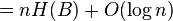
Analysis of RRR:
- Let S be a string in which a occurs n_a times
- Its entropy is H(S) = sum_a \frac{n_a}{n} \log \frac{n}{n_a}
- let x_i be the number of 1s in block i, let n_1 be the overall number of 1s, i.e.
-

-

-
 (choice of x_i in each block is subset of choice of n_1 overall)
-
![\lg {n \choose n_{1}}=[\ln(n!)-\ln(n_{1}!)-\ln(n_{0}!))]/\ln(2)](vpds-archiv_files/37567c8ea7b8234e50e91ce5b70e6f53.png)
-
![=[n\ln(n)-n-n_{1}\ln(n_{1})+n_{1}-n_{0}\ln n_{0}+n_{0}+O(\log n)]/\ln(2)](vpds-archiv_files/80018e889469da04a42c3e6df1a54cb2.png)
-
 (linear terms cancel out, n\ln(n) divided into two parts: n_0\ln(n) and n_1\ln(n))
-
Use in wavelet tree (see Navarro survey of wavelet trees):
- top level n0 zeroes, n1 ones, level 1: n00, n01, n10, n11
- top level entropy encoding uses n0 lg(n/n0) + n1 lg(n/n1) bits
- next level uses n00 lg(n0/n00) + n01 lg(n0/n01) + n10 lg(n1/n10) + n11 lg(n1/n11)
- add together n00 lg(n/n00) + n01 lg(n/n01) + n10 lg(n/n10) + n11 lg(n/n11)
- continue like this until you get sum_c n_c lg(n/n_c) which is nH(T)
Instead of wavelet tree, store indicator vector for each character from alphabet in RRR string
-
![\sum _{a}[n_{a}\lg {\frac {n}{n_{a}}}+(n-n_{a})\lg {\frac {n}{n-n_{a}}}+o(n)]](vpds-archiv_files/e181bd123861abaead498500c0655320.png)
- the first terms in the sum equal to n H(T), the last terms sum to
 , middle terms can be bound by O(n)
-

- We have used inequality ln(1+x)<=x for x>=-1
- Then

Binarny strom
- pridame pomocne listy tak, aby kazdy povodny vrchol bol vnut vrchol s 2 detmi
- ak sme mali n vrcholov, teraz mame n vnut. vrcholov a n+1 listov, t.j. 2n+1 vrcholov
- ocislujeme ich v level-order (prehladavanie do sirky) cislami 1..2n+1
- vrchol je reprezentovany tymto cislom
- datova struktura: bitovy vektor dlzky 2n+1, ktory ma na pozicii i 1 prave vtedy ak vrchol i je vnutorny vrchol
- nad tymto vektorom vybudujeme rank/select struktury v o(n) pridavnej pamati
  1  2  3  4  5  6  7  8  9 10 11 12 13 14 15 16 17
  1  1  1  1  1  0  1  0  0  1  1  0  0  0  0  0  0
  A  B  C  D  E  .  F  .  .  G  H  .  .  .  .  .  .
Lemma: Pre i-ty vnutorny vrchol (i-ta jednotka vo vektore, na pozicii select(i)) su jeho deti na poziciach 2i a 2i+1
- indukcia na i
- pre i=1 (koren) ma deti na poziciach 2 a 3
- deti i-teho vnutorneho vrcholu su v poradi hned po detoch (i-1)-veho
- dva pripady podla toho, ci (i-1)-vy a i-ty su na tej istej alebo
roznych urvniach, ale v oboch pripadoch medzi nimi len pomocne listy a
teda medzi ich detmi nic (obrazok)
- kedze deti (i-1)-veho su na poziciach podla IH 2i-2 a 2i-1, deti i-teho budu na 2i a 2i+1.
Dosledok:
- left_child(i) = 2 rank(i)
- right_child(i) = 2 rank(i)+1
- parent(i) = select(floor(i/2))
Ak chceme pouzit ako lexikograficky strom nad binarnou abecedou: potrebujeme zistit, ci vnut. vrchol zodpoveda slovu v mnozine
- jednoduchu fix s n dalsimi bitmi: z cisla vrchola 1..2n+1 zistime
rankom cislo vnut vrchola 0..n-1 a pre kazde si pamatame bit, ci je to
slovo z mnoziny
- da sa asi aj lepsie
Catalanove cisla
Ekvivalentne problemy:
- kolko je binarnych stromov s n vrcholmi?
- kolko je usporiadanych zakorenenych stromov s n+1 vrcholmi?
- kolko je dobre uzatvorkovanych vyrazov z n parov zatvoriek?
- kolko je postupnosti, ktore obsahuju n krat +1 a n krat -1 a pre ktore su vsetky prefixove sucty nezaporne?
Chceme dokazat, ze odpoved je Catalanovo cislo <tex>C_n =
{2n\choose n}/(n+1)</tex> (C_0 = 1, C_1=1, C_2 = 2, C_3 = 5,...)
- Rekurencia <tex>T(n) = \sum_{i=0}^{n-1}
T(i)T(n-i-1)</tex> (nech najlavejsia zatvorka obsahuje vo vnutri i
parov), riesime metodami kombinatorickej analyzy (generujuce funkcie)
- Iny dokaz [30]
- Nech X(n,m,k) je mnozina vsetkych postupnosti dlzky n+m obsahujucich n +1, m -1 a takych ze kazdy prefixovy sucet je aspon k.
-
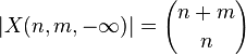
- my chceme |X(n,n,0)|
- nech Y = X(n,n,-infty)-X(n,n,0), t.j. vsetky zle postupnsti
- najdeme bijekciu medzi Y a X(n-1,n+1,-infty)
- vezmime postupnost z Y, najdime prvy zaporny prefixovy sucet (-1),
od toho bodu napravo zmenme znamienka, dostavame postupnost z
X(n-1,n+1,-infty) (obrazkovy dokaz so schodmi)
- naopak vezmime postupnost z X(n-1,n+1,-infty), najdeme prvy bod,
kde je zaporny prefixovy sucet (-1), od toho bodu napravo zmenme
znamienka, dostavame postupnost z Y
- tieto dve zobrazenia su navzajom inverzne, preto musi ist o bijekciu
- preto

-

Connection to FM index (to be covered later in the course)
- Retazec dlzky n nad abecedou velkosti sigma mozeme ulozit pomocou n
lg sigma bitov (predpokladajme pre jednoduchost, ze sigma je mocnina 2)
- napr pre binarny retazec potrebuje n bitov
- Sufixove pole na umoznuje rychlo hladat vzorku, ale potrebuje n lg n
bitov, pripadne 3 n lg n, co je rychlejsie rastuca funkcia ako n
- sufixove stromy maju tiez Theta(n log n) bitov s vacsou konstantou
- vedeli by sme rychlo vyhladavat vzorku aj s ovela mensim indexom?
- oblast uspornych datovych struktur
Back to FM index
- jednoducha finta na zlepsenie pamate pre rank:
- ulozime si rank len pre niektore i, zvysne dopocitame na zaklade pocitania vyskytov v L (vydelime pamat k, vynasobime cas k)
- rank + L pomocou wavelet tree v n lg sigma + o(n log sigma) bitoch, hladanie vyskytov sa spomali na O(m log sigma)
- ako kompaktnejsie ulozit SA
- mozeme ulozit SA len pre niektore riadky, pre ine sa pomocou LF transformacie dostaneme k najblizsiemu riadku pre ktory mame SA
- let us say we want to print SA[i], but it is not stored, let denote its unknown value x
- L[i] is T[x-1]
- let j = LF[i], j is the row in which SA[j]=x-1
- if SA[j] stored, return SA[j]+1, otherwise continue in the same way
- ako presne ulozit "niektore riadky" ked su nerovnomerne rozmiestnene v SA (rovnomerne v T)?
- samotne L mozeme ulozit aj komprimovane s vhodnymi indexami, vid.
clanok od F a M alebo ho mame reprezentovane implicitne vo wavelet tree
Opakovanie, amortizovaná zložitosť
tieto poznamky este neexistuju, mozne je ich vytvorit preklopenim informacie z prezentacie
Prioritné rady
Nizsie su pracovne poznamky, ktore doplnuju informaciu z prezentacie, je mozne ich rozsirit, doplnit samotnou prezentaciou
Introduction to priority queues
Review
Operations        Bin. heap    Fib. heap
                  worst case    amortized
MakeHeap()            O(1)       O(1)
Insert(H, x)       O(log n)      O(1)
Minimum(H)            O(1)       O(1)
ExtractMin(H)      O(log n)    O(log n)
Union(H1, H2)         O(n)       O(1)
DecreaseKey(H, x, k)
                    O(log n)     O(1)
Delete(H, x)        O(log n)   O(log n)
Applications of priority queues
- job scheduling on a server (store jobs in a max-based priority
queue, always select the one with highest priority - needs operations
insert and extract_min, possibly also delete -needs a handle)
- event-driven simulation (store events, each with a time when it is
supposed to happen. Always extract one event, process it and as a result
potentially create new events - needs insert, extract_min Examples:
queue in a bank or store: random customer arrival times, random service
times per customer)
- finding intersections of line segments [31]
- Bentley–Ottmann algorithm - sweepline: binary search tree of line
intersections) plus a priority queue with events (start of segment, end
of segment, crossing)
- for n segments and k intersections do 2n+k inserts, 2n+k extractMin, overall O((n+k)log n) time
- heapsort (builds a heap from all elements or uses n time insert,
then n times extract_min -implies a lower bound on time of
insert+extract_min must be at least Omega(log n) in the comparison
model)
- aside: partial sorting - given n elements, print k in sorted order -
selection O(n), then sort in O(k log k), together O(n + k log k)
- incremental sorting: given n elements, build a data structure, then
support extract_min called k times, k unknown in advance, running time a
function of k and n
- call selection each time O(kn)
- heap (binary, Fibonacci etc) O(n + k log n) = O(n + k log k)
because if k>= sqrt n, log n = Theta(log k) and of k < sqrt n,
O(n) term dominates
- Kruskal's algorithm (can use sort, but instead we can use heap as
well, builds heap, then calls extract_min up to m times, but possibly
fewer, plus needs union-find set structure) O(m log n)
- process edges from smallest weight upwards, if it connects 2 components, add it. Finosh when we have a tree.
- Prim's algorithm (build heap, n times extract-min, m times
decrease_key - O(m log n) with binary heaps, O(m + n log n) with Fib
heaps)
- build a tree starting from one node. For each node outside tree keep the best cost to a node in a tree as a priority in a heap
- Dijkstra's algorithm for shortest paths (build heap, n times extract_min, m times decrease_key = the same as Prim's)
- keep nodes in a heap which do not have final distance. Set the
distance of minimum node to final, update distances of tis neighbors
Soft heap
- http://en.wikipedia.org/wiki/Soft_heap
- Chazelle, B. 2000. The soft heap: an approximate priority queue with optimal error rate. J. ACM 47, 6 (Nov. 2000), 1012-1027.
- Kaplan, H. and Zwick, U. 2009. A simpler implementation and
analysis of Chazelle's soft heaps. In Proceedings of the Nineteenth
Annual ACM -SIAM Symposium on Discrete Algorithms (New York, New York,
January 4––6, 2009). Symposium on Discrete Algorithms. Society for
Industrial and Applied Mathematics, Philadelphia, PA, 477-485. pdf
- provides constant amortized time for insert, union, findMin, delete
- but corrupts (increases) keys of up to epsilon*n elements, where
epsilon is a fixed parameter in (0,1/2) and n is the number of
insertions so far
- useful to obtain minimum spanning tree in O(m alpha(m,n)) where alpha is the inverse of Ackermann's function
Fibonacci heaps
Motivation
- To improve Dijkstra's shortes path algorithm from O(E*log V) to O(E + V*log V)
Structure of a Fibonacci heap
- Heap is collection of rooted trees, node degrees up to Deg(n) = O(log n)
- Min-heap property: Key in each non-root node ≥ key in its parent
- In each node store: key, other data, referrence for parent, first child, next and previous sibling, degree, binary mark
- In each heap: number of nodes n, pointers for: root with minimum key, first and last root
- Roots in a heap are connected by sibling pointers
- Non-root node is marked iff it lost a child since getting a parrent
- Potential function: number of roots + 2 * number of marked nodes

Example of Fibonacci heap
Operations analysis
- n number of nodes in heap
- Deg(n) - maximum degree of a node x in a heap of size n
- potential function Φ = number of roots + 2 * number of marked nodes
- Amortized cost = real cost + Φ_after- Φ_before
Lazy operations with O(1) amortized time:
MakeHeap()
- create empty heap
- cost O(1), Φ= 0
- initialize H.n = [], H.min = null
Insert(H,x)
- insert node with value x into heap H:
- create new singleton node
- add this node to left of minimum pointer - update H.n
- update minimum pointer - H.min
- cost O(1), Φ= 1
Minimum(H)
- return minimum value from heap H - update H.min
- cost O(1), Φ= 0
Union(H1, H2)
- union two heaps
- concatenate root lists - update H.n, H.min
- cost O(1), Φ = 0
Other operations
ExtractMin(H)
- from heap H remove node with minimum value
- let x be root node with minimum key value, then it is in root list, and we have on him H.min pointer
- if x is singleton node (with no children), we will just extract him, return H.min and run consolidate(H) to find new H.min
- if x had children, before extracting x, we must add all children of
x to root list, update their parent pointer, then return H.min and run
then consolidate(H) to find new H.min
- what do consolite(H): changes structure of heap to achieve that no two nodes in root list have same degree, and finds H.min
- during one iteration througth root list, for each node in root list
it creates pointer to degree array, when it find two nodes with same
degree, it will link them together (HeapLink), thus node with higher key
value will be first left child of node with lower degree, also during
this iteration it is finding H.min
Analysis:
- t1 original count of nodes in the root list, t2 new count
- actual cost: O(Deg(n) + t1)
- O(Deg(n)) adding x's children into root list and updating H.min
- O(Deg(n) + t1) consolidating trees - computating is proportional to
size of root list, and number of roots decreases by one after each
merging (HeapLink)
- Amortized cost: O(Deg(n))
- t2 ≤ Deg(n) + 1, because each tree had different degree
- Δ Φ ≤ Deg(n) + 1 - t1
- let c be degree of z, c ≤ Deg(n) = O(log n)
- ExtractMin: adding children to root list: cost c, Δ Φ = c
- Consolidate: cost: t1 + Deg(n), Δ Φ = t2 - t1
- amortized t2 + Deg(n), but t2 ≤ Deg(n), therefore O(log n)
- Heaplink: cost 0, Φ = 0
1 ExtractMin (H) {
2   z = H.min
3   Add each child of z to root list of H ( update its parent )
4   Remove z from root list of H
5   Consolidate (H)
6   return z
7 }
1 Consolidate (H) {
2   create array A [ 0..Deg(H.n ) ], initialize with null
3   for (each node x in the root listt of H) {
4     while (A[x.degree] != null ) {
5       y = A[x.degree] ;
6       A[x.degree] = null ;
7       x = HeapLink (H, x, y)
8     }
9   A[x.degree] = x
10  }
11  traverse A, create root list of H, find H.min
12 }
1 HeapLink (H, x, y) {
2   if (x.key > y.key) exchange x and y
3   remove y from root list of H
4   make y a child of x, update x.degree
5   y.mark = false ;
6   return x
7 }
DecreaseKey(H,x,k)
- target: for node x in heap H change key value to k (it is decrease operation, so new value k must be lower than old value)
- find x and change it's kye value to k, there are three scenarios:
- 1. case: after changing key value for x, heap property is not
changed = value of node will be still higher than value of it's parent,
then update H.min
- 2. case: new value of node x break min-heap property and parent y (for node x) is not marked (hasn't yet lost a child), then cut link between x and y, mark y (now he lost child) and tree x add to root list, update H.min
- 3. case: new value of node x break min-heap property and parent y (for node x) is marked
(in history of heap he lost child), then cut link between x and y, tree
x add to root list (similar to previous 2. case, but...), cut link
between y and its parent z, add tree y to root list, and continue
recursively
- unmark each marked node added into root list
Analysis:
- t1 original count of nodes in the root list, t2 count of nodes in new heap
- m1 original count of marks in H, m2 count of marks in new heap
- Actual cost: O(c)
- O(1) for changing key value
- O(1) for each c cascading cuts and adding into root list
- Change in potential: O(1) - c
- t2 = t1 + c (adding c trees to root list)
- m2 ≤ m1 -c + 2 (every marked node, that was cuted was unmarked in root list, but last cut could posibly mark a node)
- Δ Φ ≤ c + 2*(-c + 2) = 4 - c
- Amortized cost: O(1)
DecreaseKey (H, x, k) {
2   x.key = k
3   y = x.parent
4   if (y != NULL && x.key < y.key) {
5     Cut(H, x, y)
6     CascadingCut (H, y)
7   }
8   update H.min
9 }
1 CascadingCut (H, y) {
2   z = y.parent
3   if (z != null) {
4     if (y.mark==false) y.mark = true
5     else {
6       Cut(H, y, z) ;
7       CascadingCut(H, z)
8     }
9   }
10 }
Delete(H,x)
- remove node x from heap H
- DecreaseKey(H,x, -infinity)
- ExtractMin(H)
- O(log n) amortized
Maximum degree Deg(n)
Proof of Lemma 3:
- Linking done only in Consolidate for 2 roots of equal degree.
- When y_j was linked, y_1,...y_{j-1} were children, so at that time x.degree >= j-1.
- Therefore at that time y_j.degree>= j-1
- Since then y_j lost at most 1 child, so y_j.degree >= j=2.
Proof of Lemma 4:
- Let D(x) be the size of subtree rooted at x
- Let s_k be the minimum size of a node with degree k in any Fibonacci heap (we will prove
 )
)
- s_k<= s_{k+1}
- If we have a subtree of degree k+1, we can cut it from its parent and then cut away one child to get a smaller tree of degree k
- Let x be a node of degree k and size s_k
- Let y_1,...y_k be its children from earliest
- D(x) = s_k = 1 + sum_{j=1}^k D(y_j) >= 1 + D(y_1) + sum_{j=2}^k s_{y_j.degree}
- >= 2 + sum_{j=2}^k s_{j-2} (lemma 3)
- by induction on k: s_k >= F_{k+2}
- for k=0, s_0 = 1, F_2 = 1
- for k=1, s_1 = 2, F_3 = 1
- assume k>=2, s_i>=F_{i+2} for i<=k-1
- s_k >= 2+ sum_{j=2}^k s_{j-2} >= 2 + sum_{j=2}^k F_j (IH)
- = 1 + sum_{j=0}^k F_j = F_{k+2} (lemma 1)
Proof of Corollary:
- let x be a node of degree k in a Fibonacci heap with n nodes
- by lemma 4 n >= Φ^k
- therefore k<= log_Φ(n)
Exercise
- What sequence of operations will create a tree of depth n?
- Alternative delete (see slides)
Sources
- Michael L. Fredman, Robert E. Tarjan. "Fibonacci heaps and their
uses in improved network optimization algorithms."Journal of the ACM
1987
- Cormen, Thomas H., Charles E. Leiserson, Ronald L. Rivest, and Clifford Stein. Introduction to Algorithms. MIT Press 2001
Pairing heaps
- Simple and fast in practice
- hard to analyze amortized time
- Fredman, Michael L.; Sedgewick, Robert; Sleator, Daniel D.; Tarjan,
Robert E. (1986), "The pairing heap: a new form of self-adjusting
heap", Algorithmica 1 (1): 111–129
- Stasko, John T.; Vitter, Jeffrey S. (1987), "Pairing heaps:
experiments and analysis", Communications of the ACM 30 (3): 234–249
- Moret, Bernard M. E.; Shapiro, Henry D. (1991), "An empirical
analysis of algorithms for constructing a minimum spanning tree", Proc.
2nd Workshop on Algorithms and Data Structures, Lecture Notes in
Computer Science 519, Springer-Verlag, pp. 400–411
- Pettie, Seth (2005), "Towards a final analysis of pairing heaps",
Proc. 46th Annual IEEE Symposium on Foundations of Computer Science, pp.
174–183 [32]
- a tree with arbitrary degrees
- each node pointer to the first child and next sibling (for delete
and decreaseKey also pointer to previous sibling or parent if first
child)
- each child has key >= key of parent
- linking two trees H1 and H2 s.t. H1 has smaller key:
- make H2 the first child of H1 (original first child of H1 is sibling of H2)
- subtrees thus ordered by age of linking from youngest to oldest
- extractMin is the most complex operation, the rest quite lazy
- insert: make a new tree of size 1, link with H
- union: link H1 and H2
- decreaseKey: cut x from its parent, decrease its key and link to H
- delete: cut x from parent, do extractMin on this tree, then link result to H
ExtractMin
- remove root, combine resulting trees to a new tree (actual cost up to n)
- start by linking pairs (1st and 2nd, 3rd and 4th,...), last may remain unpaired
- finally we link each remaining tree to the last one, starting from next-to-last back to the first (in the opposite order)
- other variants of linking were studied as well
O(log n) amortized time can be proved by a similar analysis as in splay trees (not covered in the course)
- imagine as binary tree - rename first child to left and next sibling to right
- D(x): number of descendants of node x, including x (size of a node)
- r(x): lg (D(x)) rank of a node
- potential of a tree - sum of ranks of all nodes
- details in Fredman et al 1986
- Better bounds in Pettie 2005: amortized O(log n) ExtractMin;
O(2^{2\sqrt{log log n}}) insert, union, decreaseKey; but decreaseKey not
constant as in Fibonacci heaps)
Meldable heaps (not covered in the course)
- Advantages of Fibonacci compared to binary heap: faster decreaseKey (important for Prim's and Dijkstra's), faster union
- meldable heaps support O(log n) union, but all standard operations
run in O(log n) time (except for build in O(n) and min in O(1))
- three versions: randomized, worst-case, amortized
- all of them use a binary tree similar to binary heap, but not always fully balanced
- min-heap property: key of child >= key of parent
- key operation is union
- insert: union of a single-node heap and original heap
- extract_min: remove root, union of its two subtrees
- delete and decreaseKey more problematic, different for different versions, need pointer to parent
- delete: cut away a node, union its two subtrees, hang back, may need some rebalancing
- decrease_key: use delete and insert (or cut away a node, decrease its key, union with the original tree)
Random meldable heap
Union(H1, H2) {
    if (H1 == null) return H2;
    if (H2 == null) return H1;
    if (H1.key > H2.key) { exchange H1 and H2 }
    // now we know H1.key <= H2.key
    if (rand() % 2==1) {
       H1.left = merge(H1.left, H2);
    } else {
       H1.right = merge(H1.right, H2);
    }
    return H1;
}
Analysis:
- random walk in each tree from root to a null pointer (external node)
- in each recursive call choose H1 or H2 based on key values, choose direction left or right randomly
- running time proportional to the sum of lengths of these random walks
Lemma: The expected length of a random walk in a any binary tree with n nodes is at most lg(n+1).
- let W be the length of the walk, E[W] its expected value.
- Induction on n. For n=0 we have E[W] = 0 = lg(n+1). Assume the lemma holds for all n'<n
- Let n1 be the size of the left subtree, n2 the size of right subtree. n = n1 + n2 + 1
- By the induction hypothesis E[W] <= 1 + (1/2)lg(n1+1) + (1/2)lg(n2+1)
- lg is a concave function, meaning that (lg(x)+lg(y))/2 <= lg((x+y)/2)
- E[W] <= 1 + lg((n1+n2+2)/2) = lg(n1+n2+2) = lg(n+1)
Corollary: The expected time of Union is O(log n)
A different proof of the Lemma via entropy
- add so called external nodes instead of null pointers
- let di be the depth of ith external node
- binary tree with n nodes has n+1 external nodes
- probability of random walk reaching external node i is pi = 2^{-di}, and so di = lg(1/pi)
- E[W] = sum_{i=0}^n d_i p_i = sum_{i=0}^n p_i lg(1/pi)
- we have obtained entropy of a distribution over n+1 values which is at most lg(n+1)
Leftist heaps
- Mehta and Sahni Chap. 5
- Crane, Clark Allan. "Linear lists and priority queues as balanced binary trees." (1972) (TR and thesis)
- let s(x) be distance from x to nearest external node
- s(x)=0 for external node x and s(x) = min(s(x.left), s(x.right))+1 for internal node x
- height-biased leftist tree is a binary tree in which for every internal node x we have s(x.left)>=s(x.right)
- therefore in such a tree s(x) = s(x.right)+1
Union(H1, H2) {
    if (H1 == null) return H2;
    if (H2 == null) return H1;
    if (H1.key > H2.key) { exchange H1 and H2 }
    // now we know H1.key <= H2.key
    HN = Union(H1.right, H2);
    if(H1.left != null && HN.left.s <= H1.s) {
       return new node(H1.data, H1.left, HN)
    } else {
       return new node(H1.data, HN, H1.left)
    }
}
- note: s value kept in each node, recomputed in new node(...) using s(x) = s(x.right)+1
- recursion descends only along right edges
Lemma: (a) subtree with root x has at least 2^{s(x)}-1 nodes (b) if a
subtree with root x has n nodes, s(x)<=lg(n+1) (c) the length of the
path from node x using only edges to right child is s(x)
- (a) all levels up to s(x) are filled with nodes, therefore the number of nodes is at least 1+2+4+...+2^{s(x)-1} = 2^{s(x)}-1
- (b) an easy corollary of a (n>=2^s-1 => s<-lg(n+1))
- (c) implied by height-biased leftist tree property (in each step to the right, s(x) decreases by at least 1)
Corollary: Union takes O(log n) time
- recursive calls along right edges from both roots - at most s(x)<=lg(n+1) such edges in a tree of size n
Skew Heaps
- self-adjusting version of leftist heaps, no balancing values stored in nodes
- Mehta and Sahni Chap. 6
Union(H1, H2) {
    if (H1 == null) return H2;
    if (H2 == null) return H1;
    if (H1.key > H2.key) { exchange H1 and H2 }
    // now we know H1.root.key <= H2.root.key
    HN = Union(H1.right, H2);
    return new node(H1.data, HN, H1.left)
}
Recall: Heavy-light decomposition from Link/cut trees
- D(x): number of descendants of node x, including x (size of a node)
- An edge from v to its parent p is called heavy if D(v)> D(p)/2, otherwise it is light.
Observations:
- each path from v to root at most lg n light edges because with each
light edge the size of the subtree goes down by at least 1/2
- each node has at most one child connected to it by a heavy edge
Potential function: the number of heavy right edges (right edge is an edge to a right child)
Amortized analysis of union:
- Consider one recursive call. Let left child of H1 be A, right child B
- Imagine cutting edges from root of H1 to it children A and B before
calling recursion and creating new edges to Union(B,H2) and A after
recursive call
- Let real cost of one recursive call be 1
- If edge to H1.B was heavy
- cutting edges has delta Phi = -1
- adding edges back does not create a heavy right edge, therefore delta Phi = 0
- amortized cost is 0
- If edge to H1.B was light
- cutting edges has delta Phi = 0
- adding edges creates at most one heavy right edge, therefore delta Phi <= 1
- amortized cost is <= 2
All light edges we encounter in the algorithm are on the rightmost
path in one of the two heaps, which means there are at most 2 lg n of
them (lg n in each heap). This gives us amortized cost at most 4 lg n.
Amortizované vyhľadávacie stromy a link-cut stromy
Predbežná verzia poznámok, nebojte sa upravovať: pripojiť informácie z prezentácie, pridať viac vysvetľujúceho textu a pod.
Scapegoat trees
Introduction
- Lazy amortized binary search trees
- Relatively simple to implement
- Do not require balancing information stored in nodes (needs only left child, right child and key)
- Insert and delete O(log n) amortized
- Search O(log n) worst-case
- Height of tree always O(log n)
- For now let us consider only insert and search
- Store the total number of nodes n
- Invariant: keep the height of the tree at most

- Note: 3/2 can be changed to 1/alpha for alpha in (1/2,1)
- Let D(v) denotes the size (the number of nodes) of subtree rooted at v
Insert
- Start with a usual insert, as in unbalanced BST
- If a node inserted at higher depth, restructure as follows
- Follow the path back from inserted node x to the root
- Find the first node u on this path and its parent p for which D(u)/D(p) > 2/3
- This means that node p is very unbalanced - one of its children containing more than 2/3 of the total subtree size
- Node p will be called the scapegoat
- We will show later that a scapegoat always exists on the path to root (Lemma 1)
- Completely rebuild subtree rooted at p so that it contains the same values but is completely balanced
- This is done by traversing entire subtree in inorder, storing keys in an array (sorted)
- Root of the subtree will be the median of the array, left and right subtrees constructed recursively
- Running time O(D(p))
- This can be also done using linked lists built from right pointers in the node, with only O(log n) auxiliary memory for stack
- The height was before violated by 1, this improves it at least by 1, so the invariant is satisfied
- Why we always get improvement by at least 1:
- Let v be a sibling of u, if no sibling set D(v)=0
- D(u) > 2D(p)/3 > D(p)/3 >= D(p)-D(u), do D(p)-D(u)<=D(u)-1
- D(v) = D(p)-D(u)-1 <= D(u)-2
- so the sizes of left and right subtree of p differ by at least 2
- Let height of D(u) be h. The last level contains only the last inserted node, so D(u)-1 nodes can fit to h-1 levels
- In the rebuilt tree, the size of left and right subtree will differ
by at most 1 and thus both will have at most D(u)-1 nodes and so they
can fit into h-1 levels; the hight will thus decrease by at least 1
- Finding the scapegoat also takes O(D(p)) because we need to compute D(v) at every visited node
- Each computation in time O(D(v))
- But up to node u, child has always size at most 2/3 of parent
- Therefore sizes of subtrees for which we compute D(v) grow
exponentially (geometric sum) and are dominated by the last 2
computations of D(u) and D(p)
- TODO: formulate lemma to imply both this and Lemma 1
Lemma 1: If a node x in a tree with n nodes is in depth greater than , then on the path from x to the root there is a node u and it parent p such that D(u)/D(p) > 2/3
Proof:
- Assume that this is not the case, let nodes nodes on the path from x
to root be v_k, v_{k-1},...v_0, where v_k=x and v_0 is the root and

- D(v_0) = n.
- Since D(v_i)<=2/3 D(v_{i-1}), we have D(v_i) <= (2/3)^i n.
-

- Thus we have D(x)<1, which is a contradiction, because the subtree rooted at x contains at least one node
Amortized analysis of insert
- Potential of a node v with children x,y:
-
 if |D(x)-D(y)| <= 1 (sizes of subtrees approximately the same)
-

- Potential of tree: sum of potentials of subtrees
- Insert in depth d except rebuilding:
- real cost O(d)
- change of Phi at most 3d, because potential increases by at most 3
for nodes on the path to newly inserted vertex and does not change
elsewhere
- amortized cost O(d) = O(log n)
- Rebuilding:
- real cost m = D(p) where p is the scapegoat
- let u and v be children of p before rebuilt, D(u)>D(v)
- m = D(p)=D(u)+D(v)+1, D(u)>2m/3, D(v)<m/3, D(u)-D(v)>1/3 m
- before rebuilt Phi(p) > m-3
- potential in all nodes in the rebuilt subtree is 0
- change of Phi <= -m +3
- amortized cost O(1)
Delete
- Very lazy version
- Do not delete nodes, only mark them as deleted
- Keep counter of deleted nodes
- When more than half nodes marked as deleted, completely rebuild the whole tree without them
- Each lazy delete pays a constant towards future rebuild. At least n/2 deleted before next rebuild.
- Variant: delete nodes as in unbalanced binary tree. This never increases height. Rebuild when many nodes deleted.
Uses of scapegoat trees
Scapegoat trees are useful if nodes of tree hold auxiliary information which is hard to rebuild after rotation
- we will see an example in range trees used in geometry
- another simple example from Morin's book Open Data Structures:
- we want to maintain a sequence of elements (conceptually something like a linked list)
- insert gets a pointer to one node of the list and inserts a new node before it, returns pointer to the new node
- compare gets pointers to two nodes from the same list and decided which is earlier in the list
- idea: store in a scapegoat tree, key is the position in the list.
Each node holds the path from the root as a binary number stored in an
int (height is logarithmic, so it should fit)
- Exercise: details?
Sources
Splay trees
Intuition and examples
- if height of tree is large, search is expensive, we use potential
- potential of path-like trees should be large, balanced trees smaller
- what happens if we apply splay on a leaf on a path?
- side benefit: if we search for some nodes more often, they tend to be near the root
Amortized analysis of splaying
- real cost: number of rotations
- D(x): number of descendants of node x, including x (size of a node)
- r(x): lg (D(x)) rank of a node (lg denotes log_2)
-
- Exercise: asymptotically estimate potential of a path and balanced tree with n nodes
Lemma1 (proof later): consider one step of splaying x (1 or 2 rotations)
- let r(x) be rank of x before splaying, r'(x) after splaying
- amortized cost of one step of splaying is at most
- 3(r'(x)-r(x)) for zig-zag and zig-zig
- 3(r'(x)-r(x))+1 for zig
Lemma2: Amortized cost of splaying x to the root in a tree with n nodes is O(log n)
- Let r_i be rank of x after i steps of splaying, let k be the number of steps
- amortized cost is at most
- (use Lemma 1, +1 is from the last step of splaying)
- telescopic sum, terms cancel, we get
Theorem: Amortized cost of insert, search and delete in splay tree is O(log n)
- search:
- walk down to x, then splay x (if x not found, splay the last visited node)
- amortized cost is O(log n)
- insert:
- insert x as in normal binary search tree, then splay x.
- Inserting increase rank of all nodes on the path P from root t to x
- consider node v and its parent p on this path P
- D'(v) = 1 + D(v) <= D(p)
- r'(v) <= r(p)
- change in potential

- amortized cost of insert + splaying is thus O(log n)
- delete:
- delete x as from binary search tree (may in fact delete node for
predecessor or successor of x), then splay parent of deleted node
- deletion itself decreases potential, amortized cost of splaying is O(log n)
- amortized cost is O(log n)
- overall time in each operation proportional to the length of the
path traversed and therefore to the number of rotations done in splaying
- therefore amortized time O(log n) for each operation.
Proof of Lemma 1:
- case zig: cost 1, r'(x) = r(y), all nodes except x and y keep their ranks
- amortized cost

- case zig-zig: cost 2,
- amortized cost

- we have r'(x) = r(z), r'(y)< r'(x), r(y)> r(x)
- therefore

- therefore we need (r(x)-r'(x))+(r'(z)-r'(x))<=-2 or lg (D(x)/D'(x)) + lg (D'(z)/D'(x)) <= -2
- observe that D(x)+D'(z) <= D'(x) (in fact D'(x)=D(x)+D(z)+1 where +1 corresponds to node y)
- let a = D(x)/D'(x), b = D'(z)/D'(x), we have a+b<=1
- binary logarithm is concave, i.e. (lg(a)+lg(b))/2 <= lg((a+b)/2)
- and if a+b<=1, lg((a+b)/2) <= lg(1/2) = -1
- lg (D(x)/D'(x)) + lg (D'(z)/D'(x)) = lg a + lg b <= -2
- case zig-zag is analogous
- amortized cost

- r'(x) = r(z), r(x)<=r(y)
- therefore am. cost at most
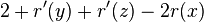
- we will prove that 2 <= 2r'(x)-r'(y)-r'(z) and this will imply amortized cost is at most 2(r'(x)-r(x))
- we have D'(y)+D'(z) <= D'(x), use the same logarithmic trick as before
Adaptability of splay trees
If some element is accessed frequently, it tends to be located near the root, making access time shorter
Weighted potential function
- Assign each node x fixed weight w(x)>0
- D(x): the sum of weights in the subtree rooted at x
- r(x) = lg(D(x)) (rank of node x)
-
Weighted version of Lemma 2:
- Amortized cost of splaying x to the root is 1+3(r(t)-r(x)) =
O(1+log (D(t)/D(x))), where t is the original root before splaying.
- Proof similar to Lemma 2
- By setting weight 1 for every node we get Lemma 2 as a corollary
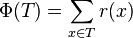
Static optimality theorem:
- Starting with a tree with n nodes, execute a sequence of m find operations, where find(x) is done q(x)>=1 times.
- The total access time is
-
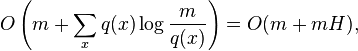
- where H is the entropy of the sequence of operations.
Proof:
- Set w(x)=q(x)/m. In weighted Lemma 2, w(T)<=1, D(x)>=w(x)=q(x)/m.
- Amortized cost of splaying x is thus O(1+log(m/q(x))); this is done q(x) times.
- After summing this expression for all operations we get the stated bound.
- However, we have to add a decrease of potential (using up money from the bank)
- with these weights, D(x)<=1, r(x)<=0 and thus Phi(x)<=0
- on the other hand, D(x)>w(x),

-
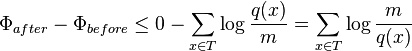
- Since q(x)>=1 and log(m/q(x))>=0, this is within stated upper bound
Note:
- Lower bound for a static tree is
 (see Melhorn 1975); our tree not static
Sequential access theorem:
- Starting from any tree with n nodes, splaying each node to the root
once in the increasing order of the keys has total time O(n).
- Proved by Tarjan 1985, improved proof Elmasry 2004 (proof not covered in the course)
- Trivial upper bound from our amortized analysis is O(n log n)
Collection of splay trees
Image now a collection of splay trees. The following operations can
be done in O(log n) amortized time (each operation gets pointer to a
node)
- findMin(v): find the minimum element in a tree containing v and make it root of that tree
- splay v, follow left pointers to min m, splay m, return m
- join(v1, v2): all elements in tree of v1 must be smaller than all elements in tree of v2. Join these two trees into one
- m = findMin(v2), splay(v1), connect v1 as a left child of m, return m
- connecting increases rank of m by at most log n
- splitAfter(x) - split tree containing v into 2 trees, one
containing keys <=x, one containing keys > x, return root of the
second tree
- splay(v), then cut away its right child and return it
- decreases rank of v
- splitBefore(v) - split tree containing v into 2 trees, one
containing keys <x, one containing keys >=x, return root of the
first tree
- analogous, cut away left child
Sources
- Sleator, Daniel Dominic, and Robert Endre Tarjan. "Self-adjusting
binary search trees." Journal of the ACM 32, no. 3 (1985): 652-686.
- Original publication of splay trees.
- Elmasry A. On the sequential access theorem and deque conjecture
for splay trees. Theoretical Computer Science. 2004 Apr
10;314(3):459-66.
- Proof of an improved version of the sequential access theorem
- Mehlhorn K. Nearly optimal binary search trees. Acta Informatica. 1975 Dec 1;5(4):287-95.
- Proof of the lower bound on static optma binary search trees (theorem 2, page 292)
Link-cut trees
Union/find
Maintains a collection of disjoint sets, supports operations
- union(v, w): connects sets containing v and w
- find(v): returns representative element of the set containing v (can be used to test of v and w are in the same set)
Can be used to maintain connected components if we add edges to the
graph, also useful in Kruskal's algorithm for minimum spanning tree
Implementation
- each set represented by a (non-binary) tree, in which each node v has a pointer to its parent v.p
- find(v) follows pointers to the root of the tree, returns the root
- union calls find for v and w and joins one with the other
- if we keep track of tree height and always join shorter tree below
higher tree plus do path compression, we get amortized time
O(alpha(m+n,n)) where alpha is inverse ackermann function, extremely
slowly growing (n = number of elements, m = number of queries)
Exercise: implement as a collection of splay trees
- hint: want to use join for union, but what about the keys?
- splay trees actually do not need to store key values if we do not search
Link/cut trees
Maintains a collection of disjoint rooted trees on n nodes
- findRoot(v) find root of tree containing v
- link(v,w) w a root, v not in tree of w, make w a child of v
- cut(v) cut edge connecting v to its parent (v not a root)
O(log n) amortized per operation. We will show O(log^2) amortized
time. Can be also modified to support these operations in worst-case
O(log n) time, add more operations e.g. with weights in nodes.
Similar as union-find, but adds cut plus we cannot rearrange trees as needed as in union-find
Simpler version for paths
Simpler version for paths (imagine them as going upwards):
- findPathHead(v) - highest element on path containing v
- linkPaths(v, w) - join paths containing v and w (head of v's path will remain head)
- splitPathAbove(v) - remove edge connecting v to its parent p, return some node in the path containing p
- splitPathBelow(v) - remove edge connecting v to its child c, return some node in the path containing c
Can be done by splay trees
- keep each path in a splay tree, using position as a key (not stored anywhere)
- findPathHead(v): findMin(v)
- linkPaths(v, w): join(v, w)
- splitPathAbove(v): splitBefore(v)
- splitPathBelow(v): splitAfter(v)
Back to link/cut trees
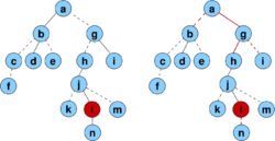
- label each edge as dashed or solid; among children of each node at most one connected by a solid edge
- series of solid paths (some solid paths contain only a single vertex)
- each solid path represented as a splay tree as above
- each node remembers the dashed edge going to its parent (if any) - only in the head of a solid path
- expose(v): make v the lower end of a solid path to root (make all
edges on the path to root solid and make other edges dashed as
necessary)
- assume for now that this can be done in O(log^2 n) amortized time
- findRoot(v): findPathHead(expose(v))
- link(v,w):
- expose(v)
- linkPaths(v, w)
- cut(v):
- expose(v) note: v not a root and thus connected to its parent by a solid edge
- splitPathAbove(v)
expose(v)
- series of splices where each splice adds one solid edge on the path from v to root
y = cutPathBellow(v);
if(y!=NULL) findPathHead(y).dashed = v;
while(true) {
  x = findPathHead(v);
  w = x.dashed;
  if(w == NULL) break;
  x.dashed = NULL;
  q = splitPathBelow(w);
  if(q != NULL) {
    findPathHead(q).dashed = w;
  }
  linkPaths(w, x); v = x;
}
- we will prove that m link-cut operations with n nodes cause O(m log
n) splices which means O(log n) splices amortized per expose
- each splice O(log n) amortized time (from splay trees), therefore O(log^2 n) amortized time per link-cut operation
Heavy-light decomposition
edge from v to its parent p is called heavy if D(v)> D(p)/2, otherwise it is light.
Observations:
- each path from v to root at most lg n light edges because with each
light edge the size of the subtree goes down by at least 1/2
- each node has at most one child connected to it by a heavy edge
Proof that there are O(log n) splices amortized per expose
- potential function: number of heavy dashed edges
- real cost: number of splices (= number of iterations of the while loop in expose)
consider a single splice, there are two cases:
- case 1: new solid edge is heavy
- before it was dashed heavy edge, not it is solid heavy edge, so potential decreases by 1
- some edge might have been changed from solid to dashed, but this edge is for sure light, because its sibling is heavy
- overall change of potential is therefore -1, real cost 1, amortized cost 0
- case 2: new solid edge is light
- change of potential is at most 1, because we might have created one new dashed edge and it is possible that this edge is heavy
- real cost is 1, therefore amortized cost is at most 2
Amortized cost of the whole expose is therefore 2L+1, where L is the number of new light solid edges created in expose
- +1 comes from the child of v which was potentially changed from solid to dashed in the first step
- all new light solid edges are light edges on the path from v to root, therefore L=O(log n)
- the total amortized cost of expose is therefore O(log n)
some operations change the tree and create new heavy dashed edges from light dashed edges
- consider edge from u to its parent p
- it can become heavy if u becomes heavier by linking in its subtree
- this never happens because edge u->p would be solid before linking
- it can also become heavy if some other child x of p becomes lighter by cutting something in its subtree
- after cutting, x is connected to p by a light edge
- there are at most lg n vertices on the path exposed by cutting that are light after the cut and can play role of x
- each x has at most one sibling u that becomes heavy
- therefore there are at most lg n new heavy dashed edges, which adds O(log n) splices to amortized cost of cut
Fully dynamic connectivity
- insert delete edges, insert delete isolated vertices, test if there is a path from v to w O(log^2 n) amortized
- Holm, Jacob, Kristian De Lichtenberg, and Mikkel Thorup.
"Poly-logarithmic deterministic fully-dynamic algorithms for
connectivity, minimum spanning tree, 2-edge, and biconnectivity."
Journal of the ACM (JACM) 48, no. 4 (2001): 723-760.
- uses link-cut trees as components
- good idea for presentation?
- if no delete, can use union-find
Applications
- At the time of publication improved best known running time of
maximum flow problem from O(nm log^2 n) to O(nm log n). Since then some
improvements.
- lca(u,v) least common ancestor:
- expose(u)
- expose(v)
- w = findPathHead(u)
- if w.dashed==null return u else return w.dashed
- we have seen O(1) lca after preprocessing a static tree, this would be O(log n) dynamic
Sources
- Sleator, Daniel D., and Robert Endre Tarjan. ``A data structure for dynamic trees. Journal of computer and system sciences 26, no. 3 (1983): 362-391.
- Sleator, Daniel Dominic, and Robert Endre Tarjan. "Self-adjusting
binary search trees." Journal of the ACM 32, no. 3 (1985): 652-686.
- Erik Demaine and his students. "Notes for Lecture 19 Dynamic
graphs" MIT course 6.851: Advanced Data Structures, Spring 2012. [37]
- Mehta, Dinesh P. and Sartaj Sahni eds. "Handbook of data structures and applications." CRC Press, 2004. Section 35.2
RMQ a LCA
Predbežná verzia poznámok, nebojte sa upravovať: pripojiť informácie z prezentácie, pridať viac vysvetľujúceho textu a pod.
Introduction to LCA, RMQ

- v is ancestor of u if it is on the path from u to the root
- lca(u,v): node of greatest depth in the intersection of the set of ancestors of u and the set of ancestors of v
- note that a node is ancestor of itself and if u is ancestor of v, then lca(u,v)=u
Task: preprocess tree T in O(n), answer lca(u,v) in O(1)
History: Harel and Tarjan 1984, Schieber a Vishkin 1988 (Gusfield book),
Bender and Farach-Colton 2000 (this lecture)
LCA via RMQ
- zname algoritmy a triv. algoritmy na slajde
- definicia poli V, D, R + ich vytvorenie slajdy
- V -- visited nodes
- D -- their depths
- R -- first occurrence of node in V
- assume that LCA(u,v) = x (fig.) and that R[u]<=R[v]
- tree traversal visits x, then subtree with u, then again x, then
subtree with v, then again x, and only after that it can get above x
- D[x] = min D[R[u]..R[v]]
- this holds even if LCA(u,v)=u (LCA(u,v) cannot be v if R[u]<R[v])
- if we can quickly find k = arg min_k in {i..j} D[k], the result is V[k]
- we have trasformed LCA to a new problem
Range minimum query RMQ
- goal: preprocess array A so that we can any two indices i and j quickly find index of minimum in A[i..j]
- Alg 1: no preprocessing, O(n) query: find minimum in interval
- Alg 2: O(n^2) preprocessing, O(1) query: precompute for all (i,j) in a table
- Alg 3: O(n log n) preprocessing, O(1) query: store minimum only for intervals of length 2^k
- M[i,k]: index of minimum in A[i..i+2^k-1] for k=1,2,...,floor(log n)
i    0  1  2  3  4  5  6  7  8  9 10 11 12
A[i] 0  1  2  1  2  3  2  1  0  1  0  1  0
--------------------------------------------
k=1  0  1  3  3  4  6  7  8  0 10 10 12  -
k=2  0  1  3  3  7  8  8  8  8 10  -  -  -
k=3  0  8  8  8  8  8  -  -  -  -  -  -  -
- Preprocessing M[i,k]: if A[M[i,k-1]]<A[M[i+2^{k-1},k-1]] then M[i,k]=M[i,k-1], else M[i,k]=M[i+2^{k-1},k-1]
- RMQ(i,j):
- let k=floor(log_2(j-i+1)) (max size of a block inside A[i..j]), floor(log x) can be precomputed for i=1..n
- if A[M[i,k]]<A[M[j-2^k+1,k]] return M[i,k] else return M[j-2^k+1,k] (figure of overlapping intervals)
+-1RMQ
- Adjacent elements of array D in LCA differ by exactly 1, i.e. 1 D[i]-D[i+1] in {-1,1}
- We will show a better RMQ data structure for arrays with this property. This problem is called +-1RMQ
- Split A into blocks of size m = lg(n)/2
- Find minimum in each block, these minima store in array A'[0..n'-1]
and position of these minima into array M'[0..n'-1] where n' = n/m =
2n/lg n
- Preprocess array A' using algorithm 3 in O(n'log n') = O(n) time
- RMQ(i,j) query considers two cases (figure):
- i and j are in different blocks bi and bj
- compute RMQ in A'[bi+1..bj-1] in O(1)
- compute minimum in block bi from i to end of block (see below)
- compute minimum in block bj from start to j (see below)
- find minimum of these three numbers
- i and j are in the same block
- compute minimum between two indices in the same block
- remains to show: how to compute +-1RMQ within blocksv ramci blokov
- representation of a block: the first element + differences between adjacent elements, e.g. 2,3,2,1 -> 2,+1,-1,-1
- na urcenie polohy minima nepotrebujeme vediet prvy prvok, staci iba m-1 rozdielov +1,-1,-1
- kazdy blok sa teda da zapisat ako binarne cislo s m-1 bitmi
- najviac 2^{m-1}<=sqrt(n) roznych typov blokov
- pre kazdy typ predpocitaj vsetky odpovede (alg. 2) v case O(m^2)
- spolu teda O(2^{m-1} m^2) = O(sqrt(n)*log(n)^2) = o(n)
+-1RMQ predpracovanie:
- spocitaj typ kazdeho bloku, uloz do pola O(n)
- pre kazdy typ spocitaj odpovede o(n) (v priemere sa jeden typ opakuje cca sqrt(n) krat, takze usetrime)
- spocitaj pole A' O(n)
- predspracuj pole A' O(n)
spolu O(n)
RMQ(i,j):
- 2x minimum v bloku O(1)
- 1x minimum v A' O(1)
spolu O(1)
LCA predspracovanie:
- prehladanie stromu a vytvorenie poli O(n)
- +-1 RMQ predspracovanie O(n)
LCA(u,v)
2 pristupy do pola R, +-1RMQ na poli D, pristup do pola V O(1)
RMQ via LCA

- vieme teda dobre riesit +-1RMQ a pomocou neho aj LCA
- vseobecne RMQ vieme riesit pomocou LCA
- z pola A vytvorime karteziansky strom:
- v koreni ma polohu i najmensieho cisla
- v lavom podstrome rekurzive definovany strom pre cast pola a[0..i-1]
- v pravom podstrome rekurzivne definovany strom pre cast pola a[i+1..n]
- RMQ(i,j) = LCA(i,j)
- vezmime si uplne minimum v poli na poz. k: pre ktore dvojice bude vyslekodm RMQ(i,j)?
- pre tie, kde i<=k, j>=k, pre tieto je k aj LCA
- ostatne dvojice su bude uplne nalavo od k alebo uplne napravo, tam je strom definovany rekurzivne a teda tiez funguje
- strom sa da vytvorit v O(n):
- ak uz mame strom pre a[0..i-1] a pridavame a[i], a[i] bude niekde na najpravejsej ceste
- ideme zo spodu po tejto ceste a najdeme prvy vrchol j, pre ktory a[j]<a[i]
- i dame ako prave dieta j, stare prave dieta j dame ako lave dieta i
- kazdy vrchol raz pridame do cesty a raz uberieme (vsetky vrcholy,
ktore sme presli pri hladani j uz nie su na pravej ceste), teda celkovo
O(n)
- potential function: number of vertices on the rightmost path
Segment trees
- root correspods to interval [0,n)
- leafs correspond to intervals of length 1, [i,i+1)
- if node corresponds to [i,j)
- left child corresponds to [i,k), right child to [k,j) where k = floor((i+j)/2)
- overall the number of nodes roughly 2n, height ceiling(lg n)
- each interval contains the result for its range (minimum, sum,...)
Decompose query interval [x,y) to a set of disjoint tree intervals (canonical decomposition):
- let current node has interval [i,j) and its left child interval [i,k)
- invariant: [i,j) overlaps with [x,y)
- if [i,j) is a subset of [x,y), include [i,j) in the decomposition and stop
- if [i,k) overlaps with [x,y), recurse on left child
- if [k,j) overlaps with [x,y), recurse on right child
Tree of recursive calls:
- sometimes recursion on only one child, sometimes both (split)
- first follow a single path from the root, each time moving to the left or right child
- last node before first split: smallest interval in the tree which contains whole [x,y), lca of leaves [x,x+1), [y,y+1)
- first split to both left and right: spliting point k inside [x,y)
- after that in the left branch [x,y) always covers right endpoint,
therefore even if we split, right recursive calls will terminate in the
next step with case 1
- similarly in the right branch [x,y) covers left endpoint, therefore left calls will terminate
- together at most 2 traversals from root to leaf plus a short call
in each step, which means at most 4 ceil(lg n) vertices visited
Segment trees can also support dynamic case where we add operation set(i,x) which sets A[i] = x
- this would require large changes in prefix sum or O(n log n) RMQ data structures
- but here only O(log n) vertices on the path from the changed leaf to the root are affected
Print small
- mame pole cisel A, predspracovane pre RMQ
- chceme vypisat vsetky indexy k in {i..j} take ze A[i]<=x
void small(i,j,x) {
  if(j<i) return;
  k = rmq(i,j);
  if(a[k]<=x) {
    print k;
    small(i,k-1);
    small(k+1,j);
  }
}
- analyzujte cas vypoctu vzhladom na p, kde p je pocet vypisanych indexov
Vyhľadávanie kľúčových slov
Predbežná verzia poznámok, nebojte sa upravovať: pripojiť informácie z prezentácie, pridať viac vysvetľujúceho textu a pod.
Keyword search, inverted index, tries, set intersection
Full-text keyword search (Plnotextove vyhladavanie klucovych slov)
- definicia problemu: slides
- zacat diskusiu o tom, co treba indexovat
- Inverted index: for each word list the documents in which it appears.
Ema: 0,2
Emu: 1
ma: 0,1,2
Mama: 1,2
mamu: 0
sa: 2
- What data structures do we need:
- Map from words to lists (e.g. sorted array, binary search tree, hash)
- List of documents for each word (array or linked list)
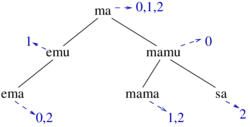
- Budeme navrhovat riesenia a analyzovat zlozitost:
- cas predspracovania, cas na jeden dotaz
- Parametre: n pocet roznych slov, N celkovy pocet vyskytov (sucet
dlzok zoznamov), m - max. dlzka slova, p - pocet najdenych vyskytov v
danom dotaze, sigma - velkost abecedy
| Štruktúra
|
query
|
preprocessing
|
| Utriedené pole
|
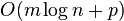
|
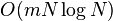
|
| Vyhľ. strom
|
|
|
| Hašovanie - najh. prípad
|

|

|
| Hašovanie - priem. prípad
|

|

|
| Lex. strom
|
|
 (neskor) (neskor)
|
Tries (lexikograficke stromy)
- A different structure for storing a collection of words
- Edges from each node labeled with characters of the alphabet (0 to |Sigma| edges)
- Each node represents a string obtained by concatenation of characters on the edges
- If this string is in the collection, the node stores pointer to the list of occurrences (or other data)
- Small alphabet 0..sigma-1: in each node array of pointers child of length sigma-1, list of occurrences (possibly empty)
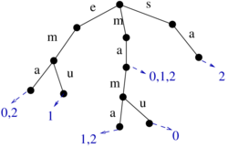
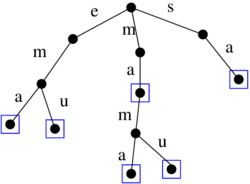
- Search for a word w of length m in the trie:
node = root;
for(i=0; i<m; i++) {
   node = node->child[w[i]];
   if(! node) return empty_list;
}
return node->list;
Time: O(m)
- Adding an occurrence of word w in document d to the trie:
node = root;
for(i=0; i<m; i++) {
   if(! node->child[w[i]]) {
     node->child[w[i]] = new node;
   }
   node = node->child[w[i]];
}
node->list.add(d)
Time: O(m) (assuming list addition in O(1))
Deletion of a word: what needs to be done (when do we delete a
vertex), possibly a problem with deletion from list of occurrences
Summary and implementations
- several words, total length D, alphabet size sigma, query size m, number of words n
- full array: memory O(D sigma), search O(m), insert all words O(D sigma)
- sorted array of variable size memory O(D), search O(m log sigma),
add one word O(m log sigma + sigma), all words O(D log sigma + n sigma)
- binary tree with letters as keywords: as before, but add only O(m log sigma)
- hashing of alphabet: on average get rid of log sigma but many practical issues (resizing...)
Multiple keywords
- Given several keywords, find documents that contain all of them (intersection, AND)
- Let us consider 2 keywords, one with m documents, other with n, m<n
- Assume that for each keyword we have a sorted array of occurrences (sorted e.g. by document ID, pagerank,...)
- Solution 1: Similar to merge in mergesort O(m+n) = O(n):
i=0; j=0;
while(i<m && j<n) {
  if(a[i]==b[j]) { print a[i]; i++; j++; }
  else if(a[i]<b[j]) { i++; }
  else { j++; }
}
What if m<<n?
for(i=0; i<m; i++) {
   k = binary_search(b, a[i])
   if(a[i]==b[k]) print k;
}
- Rewrite a little bit to get an algorithm that generalizes the two (and possibly works faster)
j = 0; // current position in b
for(i=0; i<m; i++) {
    find smallest k>=j s.t. b[k]>=a[i]; (*)
    if(k==n) { break; }
    j=k;
    if(a[i]==b[j]) {
      print a[i];
      j++;
    }
}
How to do (*):
- linear search k=j; while(k<n && b[k]<a[i]) { k++; } the same algorithm as before
- binary search in b[j..n]
 , faster for very small m
- doubling search/galloping search Bentley, Yao 1976 (general idea),
Demaine, Lopez-Ortiz, Munro 2000 (application to intersection, more
complex alg.), see also Baeza-Yates, Salinger (nice overview):
step = 1; k = j; k'=k;
while(k<n && b[k]<a[i]) {
   k'=k; k=j+step; step*=2;
}
binary search in b[k'..min(n,k)];
- If k=j+x, doubling search needs O(log x) steps
- Overall running time of the algorithm: doubling search at most m
times, each time eliminates some number of elements x_i, time
log(x1)+log(x2)+...log(xm) where x1+x2+...+xm<=n For what value of
x_i is the sum is maximized? Happens for equally sized xi's, each n/m
elements,
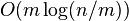 time. For constant m logarithmic, for large m linear. Also better than
simple merge if different clusters of similar values in each array.
time. For constant m logarithmic, for large m linear. Also better than
simple merge if different clusters of similar values in each array.
- If more than 2 keywords, iterate (possibly starting with smallest lists - why better?), or extend the algorithm
Sufixové stromy a polia
Predbežná verzia poznámok, nebojte sa upravovať: pripojiť
informácie z prezentácie, pridať viac vysvetľujúceho textu a pod. Cast
prednasok tu nie je zastupena, ale najdete ich v poznamkach z predmetu
Vyhľadávanie v texte - vid linka na spodku stranky.
Intro to suffix trees
- on slides
- example of generalized suffix tree for S1=aba$, S2=bba$
- at the end: uses of suffix trees (assume we can build in O(n))
- string matching - build tree, then each pattern in O(m+k) - search through a subtree - its size?
- find longest word that occurs twice in S - node with highest string depth O(n)
- find longest word that is at least two strings in input set - node
with highest string depth that has two different string represented -
how to do details O(n)
- next all maximal repeats
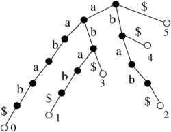

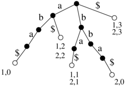
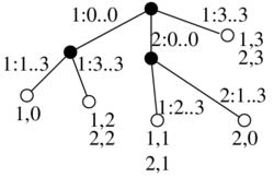
Maximal pairs
- Definition, motivation on a slide
- example: S=xabxabyabz, max pairs xab-xab, ab-ab (2x)
- Each maximal repeat is an internal node (cannot end in the middle of an edge). Why?
- Let v is a leaf for suffix S[i..n-1], let l(v)=S[i-1] - left character
- Def. Node v is diverse (roznorody) if its subtree contains leaves labeled by at least 2 different values of l(v)
- Theorem. Node v corresponds to a maximal repeat <=> v is diverse
- Proof: => obvious.
- <= Let v corresponds to string A
- v is diverse => xA, yA are substrings in S for some x!=y
- v is a node => Ap, Aq are substrings in S for some p!=q
- If xA is always followed by the same character, e.g. p, then Aq must be preceded by some z!=x, we have pairs xAp, zAq
- Otherwise we have xA is followed by at least 2 different
characters, say p and q. If yAp in S, use maximal pairs yAp, xAq,
otherwise use maximal pairs xAp, yA?
Summary
- create suffix tree for #S$
- compute l(v) for each leaf
- compute diversity of nodes in a bottom-up fashion
- print all substrings (their indices) corresponding to diverse nodes
Further extensions: find only repeats which are not parts of other repeats, finding all maximal pairs,...
LCA v sufixovych stromoch
- def na slajde
- majme listy zodpovedajuce sufixom S[i..n-1] a S[j..n-1]
- lca(u,v) = najdlhsi spolocny prefix S[i..n-1] a S[j..n-1]
- funguje aj v zovseobecnenych sufixovych stromoch, vtedy sufixy mozu byt z roznych retazcov
Aproximate string matching
- on slides, do running time analysis O(nk)
- wildcards
Counting documents
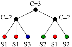
- list of leaves in DFS order
- each subtree an interval of the list
- separate to sublists: L_i = list of suffixes of S_i in DFS order
- compute lca for each two consecutive members of each L_i
- in each node counter h(v): how many times found as lca
- compute in each node l(v): number of leaves in subtree, s(v): sum of h(v) in subtree
- C(v) = l(v)-s(v)
Proof:
- consider node v and string Si
- if Si occurs k>0 times in subtree of v, it should be counted once in c(v)
- counted k-times in l(v), k-1 times in s(v)
- if Si not in subtree of v, it should be counted 0 times
- counted 0 times in both l(v) and s(v)
Printing documents
Muthukrishnan, S. "Efficient algorithms for document retrieval problems." SODA 2002. Strany 657-666.
- Preprocess texts

- Query: which documents contain pattern P?
- We can do O(m+k) where k=number of occurrences of P by simple search in suffix tree
- Using RMQ and print+small, we can achieve O(m+p) where p is the number of documents containing P
- see slides
Searching in suffix arrays
Algorithm 1
//find max i such that T[SA[i]..n] < X
L = 0; R = n;
while(L < R){
  k = (L + R + 1) / 2;
  h = 0;
  while(T[SA[k] + h] == X[h]) h++;
  if(T[SA[k]+h] < X[h]) L = k;
  else R = k - 1;
}
return L;
- O(log n) iterations
- String comparison O(m)
- Run twice: once for X=P¢, once for X=P#, where ¢ < $ < a < # for all a in the alphabet
- If the first search returns i, the second search j, patter occurrences will be at SA[i+1],...,SA[j] in T
- Counting occurrences O(m log n), printing their positions O(m log n + k), where k is the number of occurrences
Algorithm 2
Keep invariant:
- XL = lcp(T[SA[L]..n], X)
- XR = lcp(T[SA[R]..n], X)

//find max i such that T[SA[i]..n-1]< X
L = 0; R = n;
XL = lcp(X, T[SA[L]..n]); XR = lcp(X, T[SA[R]..n]);
while(R - L > 1){
  k = (L + R + 1) / 2;
  h = min(XL, XR);
  while(T[SA[k]+h]==X[h]) { h++; }
  if(T[SA[k]+h]<X[h]){ L = k; XL = h; }
  else {  R = k; XR = h; }
}
sequential search in SA[L..R];
Faster on some inputs, but still O(m log n) - see exercise
Algorithm 3
- similar to alg 2, but want to start from max(XL, XR), not min(XL, XR)
- recall that LCP(i,j) = lcp(T[SA[i]..n],T[SA[j]..n])
- assume we know LCP(i,j) for any i,j (later)
Assume XL>=XR in a given iteration (XL<XR is solved similarly. Consider three cases:
- if LCP(L,k) > XL, this imples T[SA[k]..n] < X and therefore set L=k, XL stays the same
- if LCP(L,k) < XL, this imples T[SA[k]..n] >X and therefore set R=k, XR=LCP(L,k)
- if LCP(L,k) = XL, compare X and T[SA[k]..n] starting at XL+1 (which is maximum of XL, XR)


Running time
- Overall O(log n) iterations
- each O(1) + character comparisons
- max(XL,XR) does not decrease
- overall O(log n) character comparisons ends with inequality
- character equality increases max(XL, XR) by 1
- max(XL, XR) <=m
- therefore at most m such comparisons with equality
- running time O(m+\log n)
Which LCP values are needed?

Literatúra
Burrowsova–Wheelerova transformácia
Trochu ina reverzna transformacia:
- predtym: najdi riadok j, v ktorom L[j] zodpoveda danemu F[i]
- teraz: najdi riadok j, v ktorom F[j] zopoveda danemu L[i] (toto j oznacime LF[i])
- LF[i] = C[L[i]]+ rank[L[i], i-1]
- ak riadok i zodpoveda sufixu T[k..n], tak riadok LF[i] zodpoveda sufixu T[k-1..n]
- T[n] = $; s = 0; for(i=n-1; i>=0; i--) { T[i] = L[s]; s = LF[s]; }
FM index
- Ferragina and Manzini 2000 [39]
- hladanie vyskytov P v T pomocou BWT a ranku
- T dlzky n, pripojime $ na poziciu T[n]
- zostrojime sufixove pole SA pre T a
- spocitame si rank[a,i] v L, co je pocet vyskytov znaku a v L[0..i]
- spocitame
![C[a]=\sum _{{b\in \Sigma ,b<a}}](vpds-archiv_files/ab212f62c135d61b999a718b864f34a1.png) pocet vyskytov b v T (resp. v L)
pocet vyskytov b v T (resp. v L)
- nech l(S) = najmensi index i t.z. S je prefix T[SA[i]..n]
- nech r(S) = najvacsi index ...
- pre S = epsilon, mame l(S)=0, r(S)=n
- ak aS je podslovo T, l(aS) = C[a]+rank[a,l(S)-1]
- ak aS je podslovo T, r(aS) = C[a]+rank[a,r(S)]-1
- navyse ak S je podslovo T, tak aS je podslovo T prave vtedy ak l(aS)<=r(aS)
- Opakujeme pre stale dlhsie sufixy P, nakoniec dostaneme interval SA, kde sa nachadzaju vyskyty - spatne hladanie
Priklad
hladam .ama
l(epsilon) = 0
r(epsilon) = 23
l(a) = C(a) + rank[a,L(epsilon)-1] = 6 + rank[a,-1] = 6
r(a) = C(a) + rank[a,R(epsilon)]-1 = 6 + rank[a,23]-1 = 11
l(ma) = C(m) + rank[m,L(a)-1] = 14 + rank[m,5] = 14
r(ma) = C(m) + rank[m,R(a)]-1 = 14 + rank[m,11] - 1 = 19
l(ama) = C(a) + ra(L(ma)-1) = 6 + ra(13) = 10
r(ama) = C(a) + ra(R(ma))-1 = 6 + ra(19) - 1 = 10
l(.ama) = C(.) + r.(L(ama)-1) = 1 + r.(9) =  1
r(.ama) = C(.) + r.(R(ama))-1 = 1 + r.(10)-1 =  0
Analyza
- zistovanie vyskytu, ratanie ich poctu potrebuje len polia rank a C
- na vypisanie pozicii potrebujeme aj SA
- pamat O(n sigma) cisel, pocitanie vyskytov vzorky O(m), vypis vyskytov O(m+k)
- v casti Succint data structures si ukazeme ako setrit pamat
Vyhľadávanie vzorky v texte
Literatúra
Theoretical results for edit distance computation
Exact algorithm O(mn) or improved by logarithimc factor.
Approximation algorithm: For strings of length n and every fixed ε > 0 compute  approximation in
  time
time
Source: Andoni A, Krauthgamer R, Onak K. Polylogarithmic
approximation for edit distance and the asymmetric query complexity.
FOCS2010, pp. 377-386 [41]
Conditional lower bound: If the edit distance can be computed in  for some constant δ > 0, then the satisfiability of conjunctive
normal form (CNF) formulas with N variables and M clauses can be solved
in time
for some constant δ > 0, then the satisfiability of conjunctive
normal form (CNF) formulas with N variables and M clauses can be solved
in time  for a constant
  , which would violate Strong Exponential Time Hypothesis (SETH).
Source: Backurs A, Indyk P. Edit Distance Cannot Be Computed in
Strongly Subquadratic Time (unless SETH is false). STOC2015, pp. 51-58 [42]
Hešovanie
Introduction to hashing
- Universe U = {0,..., u-1}
- Table of size m
- Hash function h : U -> {0,...,m-1}
- Let X be the set of elements currently in the hash table, n = |X|
- We will assume n = Theta(m)
Totally random hash function
- (a.k.a uniform hashing model)
- select hash value h(x) for each x in U uniformly independently
- not practical - storing this hash function requires u * lg m bits
- used for simplified analysis of hashing in ideal case
Universal family of hash functions
- some set of functions H
- draw a fuction h uniformly randomly from H
- there is a constant c such that for any distinct x,y from U we have Pr(h(x) = h(y)) <= c/m
- probability goes over choices of h
Note
- for totally random hash function, this probability is exactly 1/m
Example of a universal family:
- choose a fixed prime p >= u
- H_p = { h_a | h_a(x) =(ax mod p) mod m), 1<=a<=p-1 }
- p-1 hash functions, parameter a chosen randomly
Proof of universality
- consider x!=y, both from U
- if they collide (ax mod p) mod m = (ay mod p) mod m
- let c = (ax mod p), d = (ay mod p)
- note that c,d in {0..p-1}
- also c!=d because otherwise a(x-y) is divisible by p and both a and |x-y| are numbers from {1,...,p-1} and p is prime
- since c mod m = d mod m, then c-d = qm where 0<|qm|<p
- there are <=2(p-1)/m choices of q where |qm|<p
- we get a(x-y) mod p = qm mod p
- this has exactly one solution a in {1...p-1}
- if there were two solutions a1 and a2, then (a1-a2)(x-y) would be divisible by p, which is again not possible
- overall at most 2(p-1)/m choices of hash functions collide x and y
- out of p-1 all hash functions in H_p
- therefore probability of collision <=2/m
Hashing with chaining, using universal family of h.f.
- linked list (or vector) for each hash table slot
- let c_i be the length of chain i, let
 for x in U
- any element y from X s.t. x!=y maps to h(x) with probability <= c/m
- so E[C_x] <= 1 + n * c / m = O(1)
- from linearity of expectation - sum over indicator variables for each y in X if it collides with x
- +1 in case x is in X
- so expected time of any search, insert and delete is O(1)
- again, expectation taken over random choice of h from universal H
- however, what is the expected length of the longest chain in the table?
- O(1+ sqrt(n^2 / m)) = O(sqrt(n))
- see Brass, p. 382
- there is a matching lower bound
- for totally random hash function this is "only" O(log n / log log n)
- similar bound proved also for some more realistic families of hash functions
- so the worst-case query is on average close to logarithmic
References
Perfect hashing
Static case
- Fredman, Komlos, Szemeredi 1984
- avoid any collisions, O(1) search in a static set
- two-level scheme: use a universal hash function to hash to a table of size m = Theta(n)
- each bucket i with set of elements X_i of size c_i hashed to a
second-level hash of size m_i = alpha c_i^2 for some constant alpha
- again use a universal hash function for each second-level hash
- expected total number of collisions in a second level for slot i:
- sum_{x,y in X_i, x!=y} Pr(h(x) = h(y)) <= (c_i)^2 c/m_i = c/alpha = O(1)
- here c is the constant from definition universal family
- with a sufficently large alpha this expected number of collisions is <=1/2
- e.g. for c = 2 set alpha = 4
- then with probability >=1/2 no collisions by Markov inequality
- number of collisions is a random variable Y number with possible values 0,1,2,...
- if E[Y]<=1/2, Pr(Y>=1)<=1/2 and thus Pr(Y=0)>=1/2
- when building a hash table if we get a collision, randomly sample another hash function
- in O(1) expected trials get a good hash function
- expected space: m + sum_i m_i^2 = Theta(m + sum_i c_i^2)
- sum_i (c_i^2) is the number of pairs (x,y) s.t. x,y in X and h(x)=h(y); include x=y
-

- so expected space is linear
- can be made worst-case by repeating construction if memory too big
- expected construction time O(n)
Dynamic perfect hashing
- amortized vector-like tricks
- when a 2-nd level hash table gets too full, allocate a bigger one
- O(1) deterministic search
- O(1) amortized expectd update
- O(n) expected space
References
Bloom Filter (Bloom 1970)
- supports insert x, test if x is in the set
- may give false positives, e.g. claim that x is in the set when it is not
- false negatives do not occur
Algorithm
- a bit string B[0,...,m-1] of length m, and k hash functions hi : U -> {0, ..., m-1}.
- insert(x): set bits B[h1(x)], ..., B[hk(x)] to 1.
- test if x in the set: compute h1(y), ..., hk(y) and check whether all these bits are 1
- if yes, claim x is in the set, but possibility of error
- if no, answer no, surely true
Bounding the error If hash functions are totally random and independent, the probability of error is approximately (1-exp(-nk/m))^k
- in fact probability somewhat higher for smaller values
- proof of the bound later
- totally random hash functions impractical (need to store hash value
for each element of the universe), but the assumption simplifies
analysis
- if we set k = ln(2) m/n, get error
 .
.
-
 and thus we get error
  , where
- to get error rate p for some n, we need

- for 1% error, we need about m=10n bits of space and k=7
- memory size and error rate are independent of the size of the universe U
- compare to a hash table, which needs at least to store data items themselves (e.g. in n lg u bits)
- if we used k=1 (Bloom filter with one hash function), we need
m=n/ln(1/(1-p)) bits, which for p=0.01 is about 99.5n, about 10 times
more than with 7 hash functions
Use of Bloom filters
- e.g. an approximate index of a larger data structure on a disk - if
x not in the filter, do not bother looking at the disk, but small
number of false positives not a problem
- Example: Google BigTable maps row label, column label and timestamp
to a record, underlies many Google technologies. It uses Bloom filter
to check if a combination of row and column label occur in a given
fragment of the table
- For details, see Chang, Fay, et al. "Bigtable: A distributed
storage system for structured data." ACM Transactions on Computer
Systems (TOCS) 26.2 (2008): 4. [43]
- see also A. Z. Broder and M. Mitzenmacher. Network applications of
Bloom filters: A survey. In Internet Math. Volume 1, Number 4 (2003),
485-509. [44]
Proof of the bound
- probability that some B[i] is set to 1 by hj(x) is 1/m
- probability that B[i] is not set to 1 is therefore 1-1/m and since
we use k independent hash functions, the probability that B[i] is not
set to one by any of them is (1-1/m)^k
- if we insert n elements, each is hashed by each function
independently of other elements (hash functions are random) and thus
Pr(B[i]=0)=(1-1/m)^{nk}
- Pr(B[i]=1) = 1-Pr(B[i]=0)
- consider a new element y which is not in the set
- error occurs when B[hj(y)]==1 for all j=1..k
- assume for now that these events are independent for different j
- error then occurs with probability Pr(B[i]=1)^k = (1-(1-1/m)^{nk})^k
- recall that
- thus probability of error is approximately (1-exp(-nk/m))^k
However, Pr(B[i]=1) are not independent
- consider the following experiment: have 2 binary random variables
Y1, Y2, each generated independently, uniformly (i.e. P(Y1=1) = 0.5)
- Let X1 = Ya and X2 = Yb where a and b are chosen independently uniformly from set {1,2}
- X1 and X2 are not independent, e.g. Pr(X2 = 1|X1 = 1) = 2/3, whereas Pr(X2=1) = 1/2. (check the constants!)
- note: X1 and X2 would be independent conditioned on the sum of Y1+Y2.
- In Mitzenmacher & Upfal (2005), pp. 109–111, 308. - less strict independence assumption
Exercise
Let us assume that we have separate Bloom filters for sets A and B with
the same set k hash functions. How can we create Bloom filters for union
and intersection? Will the result be different from filter created
directly for the union or for the intersection?
Theory
- Bloom filter above use about 1.44 n lg(1/p) bits to achieve error
rate p. There is lower bound of n lg(1/p) [Carter et al 1978], constant
1.44 can be improved to 1+o(1) using more complex data structures, which
are then probably less practical
- Pagh, Anna, Rasmus Pagh, and S. Srinivasa Rao. "An optimal Bloom filter replacement." SODA 2005. [45]
- L. Carter, R. Floyd, J. Gill, G. Markowsky, and M. Wegman. Exact and approximate membership testers. STOC 1978, pages 59–65. [46]
- see also proof of lower bound in Broder and Mitzenmacher 2003 below
Counting Bloom filters
- support insert and delete
- each B[i] is a counter with b bits
- insert increases counters, delete decreases
- assume no overflows, or reserve largest value 2^b-1 as infinity, cannot be increased or decreased
- Fan, Li, et al. "Summary cache: A scalable wide-area web cache
sharing protocol." ACM SIGCOMM Computer Communication Review. Vol. 28.
No. 4. ACM, 1998. [47]
References
Locality Sensitive Hashing
- todo: expand and according to slides
- typical hashing tables used for exact search: is x in set X?
- nearest neighbor(x): find y in set X minimizing d(x,y) for a given distance measure d
- or given x and distance threshold r, find all y in X with d(x,y)<=r
- want: polynomial time preprocessing of X, polylogarithmic queries
- later in the course: geometric data structures for similar problems in R^2 or higher dimensions
- but time or space grows exponentially with dimension (alternative is linear search) - "curse of dimensionality"
- examples of high-dimensional objects: images, documents, etc.
- locality sensitive hashing (LHS) is a randomized data structure not guaranteed to find the best answer but better running time
Approximate near neighbour (r,c)-NN
- preprocess a set X of size n for given r,c
- query(x):
- if there is y in X such that d(y,x)<=r, return z in X such that d(z,x)<=c*r
- LHS returns such z with some probability at least f
Example for Hamming distance in binary strings of length d
- Hash each string using L hashing functions, each using O(log n)
randomly chosen string positions (hidden constant depends on d, r, c),
then rehash using some other hash function to tables of size O(n) or a
single table of size O(nL)
- Given q, find it using all L hash function, check every collision,
report if distance at most cr. If checked more than 3L collisions, stop.
- L = O(n^{1/c})
- Space O(nL + nd), query time O(Ld+L(d/r)log n)
- Probability of failure less than some constant f < 1, can be boosted by repeating independently
Minimum hashing
- similarity of two sets measured as Jaccard index J(A,B) = |A intersect B | / | A union B |
- distance d(A,B) = 1-J(A,B)
- used e.g. for approximate duplicate document detection based on set of words occurring in the document
- choose a totally random hash function h
- minhash_h(A) = \min_{x\in A} h(x)
- Pr(minhash_h(A)=minhash_h(B)) = J(A,B) = 1-d(A,B) if using totally random hash function an no collisions in A union B
- where can be minimum in union? if in intersection, we get equality, otherwise not
- (r_1, r_2, 1-r_1, 1-r_2)-sensitive family (if we assume no collisions)
- again can we apply amplification
Notes
- Real-valued vectors: map to bits using random projections sgn (w · x + b)
- Data-dependent hashing: Use PCA, optimization, kernel
tricks, even neural networks to learn hash functions good for a
particular set of points and distance measure (or learn even distance
measure from examples). [49]
Sources
- Har-Peled, Sariel, Piotr Indyk, and Rajeev Motwani. "Approximate
Nearest Neighbor: Towards Removing the Curse of Dimensionality." Theory
of Computing 8.1 (2012): 321-350. [50]
- Indyk and Motwani: Approximate nearest neighbors: Towards removing
the curse of dimensionality. In Proc. 30th STOC, pp. 604–613. ACM Press,
1998.
- http://www.mit.edu/~andoni/LSH/ Pointers to papers
- Wikipedia
- Several lectures:
- Charikar, Moses S. "Similarity estimation techniques from rounding algorithms." STOC 2002 [51]
Dátové štruktúry pre externú pamäť
External memory model, I/O model
Introduction
- big and slow disk, fast memory of a limited size M words
- disk reads/writes in blocks of size B words
- when analyzing algorithms, count how many disk reads/writes (memory transfers) are done
Example: scanning through n elements (e.g. to compute their sum): Theta(ceiling of n/B) memory transfers
B-trees
- I/O cost of binary search tree woth arbitray node placement?
- parameter T related to block size B (so that each node fits into a constant number of blocks)
- each node v has some number v.n of keys
- if it is an internal node, it has v.n+1 children
- keys in a node are sorted
- each subtree contains only values between two successive keys in the parent
- all leaves are in the same depth
- each node except root has at least T-1 keys and each internal node except root has at least T children
- each node has at most 2T-1 keys and at most 2T children
- height is O(log_T n)
Search:
Insert:
- find a leaf where the new key belongs
- if leaf is full (2T-1 keys), split into two equal parts of size T-1 and insert median to the parent (recursively)
- new element is inserted to one of the new leaves
- we continue splitting ancestors until we find a node which is not
full or until we reach the root. If root is full, we create a new root
with 2 children (increasing the height of the tree)
- O(log_T n) transfers
Sorting
external mergesort
- I/O cost of ordinary mergesort implementation?
- create sorted runs of size M using O(n/B) transfers
- repeatedly merge M/B-1 runs into one in 1 pass, this uses O(n/B) disk reads and writes per pass
- read one block from each run, use one block for output
- when output block gets full, write it to disk
- when some input gets exhausted, read next block from the run (if any)
- log_{M/B-1} (n/M) passes
Summary
- B-trees can do search tree operations (insert, delete,
search/predecessor) in Theta(log_{B+1} n) = Theta(log n / log (B+1))
memory transfers
- number of transfers compared to usual search tree running time: factor of 1/log B
- search optimal in comparison model
- proof outline through information theory
- goal of the search is to tell us between which two elements is query located
- there are Theta(n) possible answers, thus Theta(log n) bits of information
- in normal comparison model one comparison of query to an elements of the set gives us at most 1 bit of information
- in I/O model reading a block of B elements and comparing query to
them gives us in the best case its position within these B elements,
i.e. Theta(log B) bits
- to get Theta(log n) bits of information for the answer, we need Theta(log n/log B) block reads
- this can be transformed to a more formal and precise proof
- sorting O((n/B) log_{M/B} (n/M)) memory transfers
- number of memory transfers compared to usual sorting running time: factor of more than 1/B
- also much better than sorting using B-trees, which would take O(N * log_B n)
Cache oblivious model
Introduction
- in the I/O model the algorithm explicitly requests block transfers, knows B, controls memory allocation
- in the cache oblivious model algorithm does not know B or M, memory operates as a cache
- M/B slots, each holding one block from disk
- algorithm requests reading a word from disk
- if the block containing this word in cache, no transfer
- replace one slot with block holding requested item, write original block if needed (1 or 2 transfers)
- which one to replace: classical on-line problem of paging
Paging
- cache has size k = M/B slots, each holds one page (above called block)
- sequence of page requests, if the requested page not in memory not
in memory, bring it in and remove some other page (page fault)
- goal is to minimize the number of page faults
- optimal offline algorithm (knows the whole sequence of page requests)
- At a page fault remove the page that will not be used for the longest time
- example of an on-line algoritm: FIFO:
- at a page fault remove page which is in the memory longest time
- uses at most k times as many page faults as the optimal algorithm (k-competitive)
- no deterministic alg. can be better than k-competitive
- it is conservative: in a segment of requests containing at most k distinct pages it does at most k page faults
- proof by induction on segment length, hypothesis: each element
which was inserted within segment is never removed within segment
- every conservative alg. is k-competitive
- Compare a conservative paging alg. (e.g. FIFO) on memory with k
blocks to optimum offline alg. on a smaller memory of size h -
competitive ratio k/(k-h)
- if h = k/2, we get competitive ratio 2
- divide input sequence into maximal blocks, each containing k
distinct elements (first element of the next block is distinct from the k
elements of the previous block)
- FIFO uses at most k page faults in each block
- optimum has at most h pages from a block in memory at the beginning - at least k-h pages will cause a fault
- in fact we can prove k/(k-h+1), works even for k=h
Back to cache-oblivious model
- we analyze algorithms under the assumption that paging algorithm uses off-line optimum
- instead it could use e.g. FIFO in memory 2M and increase the number of transfers by a constant factor
- advantages of cache-oblivious model:
- may adapt to changing M, B
- good for a whole memory hierarchy (several levels of cache, disk, network,...)
- scanning still Theta(ceiling of N/B)
- search trees still Theta(log_{B+1} N)
- sorting Theta(n/B log_{M/B}(N/B)) but requires big enough M i.e. M=Omega(B^{1+epsilon})
Static cache-oblivious search trees
- first published by Harald Prokop, Master thesis, MIT 1999 [52]
- alternative to a binary search
- exercise: how many transfers for binary search?
- use perfectly balanced binary search tree
- search algorithm as usual (follows path from root down as usual)
- nodes are stored on disk in some order which we can choose
- the goal is to choose it so that for any B, M and any search we use only few blocks
- for example, what would happen if we store nodes in pre-order or level-order?
- what would be a good order for fixed known B?
- e.g. store top lg_B n levels together in one block, then split the
rest into subtrees and again store top of each subtree in a block etc.
- we do not know B, we will use van Emde Boas order which does this
recursively for several values of "B" (later in the course we will see
van Emde Boas trees for integer keys)
van Emde Boas order
- split tree of height lg n into top and bottom, each of height (1/2) lg n
- top part is a small tree with about sqrt(n) vertices
- bottom part consists of about sqrt(n) small trees, each size about sqrt(n)
- each of these small trees is processed recursively and the results are concatenated
- for example a tree with 4 levels is split into 5 trees with 2 levels, resulting in the following ordering:
          1
     2           3
  4     7    10    13
5  6  8  9 11 12 14 15
- if B = sqrt n, we need only 2 trasfers
- but we will show next that for any B<=M/2 and for any path from the root we need only Theta(log_{B+1} n) block transfers
Analysis
- k: height of trees in some level of recursion, such that size of
these trees is <=B and the next higher level has tree size >B
- (1/2) lg B <= k <= lg B
- careful: of size of these trees is x=2^k, we have sqrt(B) <= x <= B
- length of path lg n, visits lg n / k trees of height k, which is Theta(lg n / lg B)
- each tree of height k occupies at most B cells in memory (assuming
each node fits in a word, otherwise everything is multiplied by a
constant factor...)
- traversing the tree might need up to 2 memory transfers if there is
a block boundary inside interval for the tree (whole tree fits in
memory)
Dynamic cache oblivious trees
uses "ordered file maintenance"
- maintain n items in an array of size O(n) with gaps of size O(1)
- updates: delete item, insert item between given two items (similar to linked list)
- update rewrites interval of size at most O(log^2 n) amortized in O(1) scans
- done by keeping appropriate density in a hierarchy of intervals
- we will not cover details
simpler version of data structure
- our keep elements in "ordered file" in a sorted order
- build a full binary tree on top of array (segment tree)
- each node stores maximum in its subtree
- tree stored in vEB order
- when array gets too full, double the size, rebuild everything
search
- search checks max in left child and decides to move left or right
- basically follows a path from root, uses O(log_B n) transfers
update
- search to find the leaf
- update "ordered file", resulting in changes in interval of size L (L=O(log^2 n) amortized)
- then update all ancestors of these values in the tree by postorder traversal
analysis of update
- let he size of interval update in ordered file be L (amortized O(log^2 n))
- again let k be height of vEM subtrees which have size <=B but next higher level has size >B
- size of these trees is at least sqrt(B)
- (1) ordered file needs O(L/B+1) transfers
- (2) consider bottom 2 levels: O(1+L/sqrt(B)) trees of size k need updating (+1 from ceilings)
- each tree stored in <=2 blocks
- postorder traversals revisits parent block between child blocks, but if M>=4B, stays in memory
- overall O(L/sqrt(B)) transfers for bottom two layers
- (3) at the top of 2 levels, at most O(L/sqrt(B)+1) nodes, all their ancestors also need updating (set of nodes X)
- vertices have 2 children in X, some only one child
- The number of vertices with 2 children is O(L/sqrt(B)+1), this is ok, even if each causes separate transfer
- Vertices with one child are arranged in at most 2 root-to-leaf
paths, each path requires at most O(log_B n) transfers as in search
- Consider lca of all leaves in L: from root to lca, one a single
path, there splits into 2. Each node in the left path has interval with
rightmost point inside the updated interval. There are two
possibilities: (A) the right subtree is completely inside the updated
interval, which means all nodes in the right subtree 2 children inside;
the path continues left (B) the right tree is only partially inside the
updated interval, then the left subtree is outside and the path
continues right
- (1)+(2)+(3): amortized O(log^2 n / sqrt(B) + log_B n) - too big for small values of B
improvement of update
- split sorted data into buckets, each bucket of size between (1/4) lg n and lg n
- each bucket stored sequentially on disk,
- minimum element from each bucket used as a leaf in the above data structure, now contains only O(n/log n) elements
- update/search inside bucket: 1 scan, O(log n/B)
- if a bucket gets too large, split into two buckets (similarly to B-trees)
- if a bucket gets too small, connect with adjacent bucket, maybe split again more evenly
- for example, if adjacent bucket more than (1/2) lg n, split again
to get two buckets of size at least (3/8) lg n; for small adjacent
bucket get a combined bucket with size at most 3/4 lg n; in either case
at least (1/8) lg n from the end of admissible interval of bucket sizes
(1/4)lg n ad lg n.
- splitting/connecting propagates as update to the structure for n/log n items
- but this happens at most once very (1/8)lg n updates of this particular bucket, so amortized time for update divided by log n
- however, O(log_B n) term still necessary for search
Sources
Streaming model
Definition
- Input: stream of n elements
- Goal: do one pass through the stream (or only a few passes), use a
small memory (e.g. O(1) or O(log n)) and answer a specific query about
the stream
- Good for processing very fast streams, such as IP packets passing a router or measurements of a very low-powered device
- Not enough memory to store the whole stream, each item should be processed fast
- Strict turnstile model:
- underlying set {0,...,n-1}
- virtual vector F of length n initialized to zeroes
- stream consists of operations (j,x) meaning F[j]+=x
- At every point we have F[j]>=0 for each j
- Cash register model: all values x are positive
- Example: if all values x are +1, we are simply counting frequencies of elements from {0,...,n-1} on input
Majority element
Boyer–Moore majority vote algorithm 1981
- Consider the cash register model with x=1 in each update
- Assume that the stream contains a majority element j, i.e. F[j]>M/2 where M is the sum of all F[k]
- With this assumption j can be found by a simple algorithm with O(1) memory and O(1) time per element:
- Keep one candidate element j and a counter x
- Initialize j to fist element of the stream and x=1
- For each element k of the stream:
- if(j==k) x++;
- else if(x>0) x--;
- else { j=k; x=1; }
- If we are allowed a second pass, we can verify if found j is indeed majority
This algorithm can be generalized to find all elements with frequency
greater than M/k by keeping k-1 counters (Misra and Gries 1982)
- If current element has a counter, increase its counter
- Otherwise if some counter at 0, replace with current element, start at 1
- Otherwise decrease all counters by 1
- At the end the final set is guaranteed to contain all elements with frequency more than M/k (but we do not know which they are)
- Decreasing all counters is equivalent to removing k distinct
elements from the input multiset (k-1 counters plus the current element)
- The counters at the end correspond to up to k-1 distinct items on
which operation of removing k distinct elements cannot be applied - all
elements with more than M/k occurrences must be among counters
Count-Min sketch
- Strict turnstile model
- CM sketch with parameters epsilon and delta
- Array of counters A of depth
 and width
- Each row i of A has a hash function h_i from {0,...,n-1} to
{0,...,w-1} (assume totally random, but a weaker assumption of pairwise
independence sufficient for analysis)
- Update (j,x) does A[i,h_i(j)]+=x for all hash function i=0,...,n-1
- Query F[j]=? returns min_i A[i,h_i(j)]
- Let F be the correct answer, F' the answer returned
- Clearly F'>=F, because each A[i,k] may have contributions from other elements as well
- With probability at least 1-delta we have
![F'[j]\leq F[j]+\epsilon \sum _{i}F[i]](vpds-archiv_files/34dad0560ecc4efeb4be516b2898b0e4.png)
- Proof:
- Let
![M=\sum _{k}F[k]](vpds-archiv_files/080a114851fae348eafebcb7d3ecc93e.png)
- for a fixed row i:
![E[A[i,h_{i}(j)]=F[j]+\sum _{{k\neq j}}F[k]/w](vpds-archiv_files/cdfe94be7077d0d054d0194d8162c5fb.png) , because every other element k has probability 1/w to hash to column h_i(j) and thus it cntributes F[k]/w to
, because every other element k has probability 1/w to hash to column h_i(j) and thus it cntributes F[k]/w to
-
![E[A[i,h_{i}(j)]\leq F[j]+M\epsilon /e](vpds-archiv_files/e893e63da255a8c878db27a265864d42.png)
- By Markov inequality
![\Pr(A[i,h_{i}(j)]-F[j]\geq M\epsilon )\leq 1/e](vpds-archiv_files/696074ff2c3300ed9035ba634b71719a.png)
- Probability that this happens in every row i is at most

- Memory does not depend on n
- Note: if we insert million elements and then delete all but 4 of
them, in the final structure we are very likely to be able to identify
the 4 remaining ones as M is only 4
Heavy hitters
- Consider cash register model, for simplicity let all updates by simple increments by 1 (x=1)
- Let M = sum of values in F
- Given parameter phi, output all elements i from {0,...,n-1} such
that F[i]>=phi*M (we will solve this problem with approximation)
- Keep current value of M plus a CM sketch with ln(n/delta) rows
(instead of n, one could use an upper bound on M if F is very sparse)
- Also keep a hash table of elements j with current estimate
F'[j]>=phi*M for current M and a min-priority queue (binary heap) of
these elements with F'[j] as key (hash table keeps indexes within heap
of individual elements)
- After each update (j,x), get estimated F'[j] and if it is at least phi*M, add/update j in priority queue and hash table
- Also check if minimum item k in the heap has its key large enough compared to current M, otherwise remove it
- At each moment at most 1/phi elements in the heap and hash table
- Memory O(ln(n/delta)/epsilon+1/phi), time for update O(ln(n/delta)+log(1/phi))
- Theorem: Every item which occurs with count more than phi * M is
output, and with probability 1 − delta, no item whose count is less than
(phi-epsilon)M is output.
- Threshold phi*M increases in each step; the only element which may become one of heavy hitters is the one just increased
- Since count-min sketch gives upper bounds, no heavy hitter is ommitted
- For each individual element j we have Pr(F'[j]-F[j]>=epsilon*M) <= delta/n
- By union bound Pr(exists j such that F'[j]-F[j]>=epsilon*M) <= delta
- So with prob >= 1-delta for every j such that F[j]<(phi-epsilon)*M, we have F'[j]<Phi*M
Sources
- Presentation at AK Data Science Summit - S. Muthu Muthukrishnan 2013 Count-Min Sketch 10 years later video, slides
- Cormode G, Muthukrishnan S. An improved data stream summary: the
count-min sketch and its applications. Journal of Algorithms. 2005 Apr
1;55(1):58-75. [53]
- Journal article with count-min sketch
- Muthukrishnan S. Data streams: Algorithms and applications.
Foundations and Trends in Theoretical Computer Science. 2005 Sep
27;1(2):117-236. [54]
- Survey of streaming model results, count-min sketch starts at page 26
- Cormode, Graham, and Marios Hadjieleftheriou. "Finding the frequent
items in streams of data." Communications of the ACM 52.10 (2009):
97-105. [55]
- Survey and empirical comparison, include Boyer-Moore as well as count-min sketch
- Wikipedia Count-min sketch, Streaming algorithms, Boyer-Moore algorithm
Dátové štruktúry pre celočíselné kľúče
Introduction
- data structures that work only with integers
- can be used to solve predecessor problem
- van Emde Boas data structure, x-fast trees
Models of computations
- for integer data structures
- word - w-bit integer (unsigned)
- words are over universe
 of size
- all input, output, queries, ... are with respect to w-bit words
- memory is an array of words of some fixed size
Word RAM model
- word Random Access Machine
- standard model, it will be used in this lecture
- memory is divided into S cells of size w
- words can serve as pointers
- it is practical to assume
 , otherwise we can't index whole memory
- if n is the problem size, it implies

- processor may use in
 time following 'C-style' operations:
Other models
- there exist other models used with (not only) integer data structures
- transdichotomous RAM model
- almost same as word RAM, but it can have perform arbitrary operations that access at most memory cells
- cell probe model
- reading and writing costs 1, other operations are free
- unrealisitic, used for lower bounds
- pointer machine, etc.
Predecessor problem
- maintain a set S of n words over universe U
- support following operations:
- insert an element of universe into set
- delete an element of set
- find the predecessor of an element from universe in S,

- find the succecessor of an element from universe in S,

van Emde Boas data structure
- structure to solve predecessor problem
- reinterpreted version by Bender and Farach-Colton
-
 time per operation,
  space
space
- assuming n is not not much smaller compared with u, namely if
 , we get running time
  compared to
  with balanced binary search trees
- goal is to bound all operations by recurrence
 , so running time will be (e.g. by Master theorem applied to
  )
) 
- main idea is to split universe U into
 clusters, each of size

Hierarchical coordinates
- suppose we have universe of size u
- for word x, we will write
 , where:
-
 is cluster containing x
-
 is x's index within cluster
-
- if we have binary numbers:
- just split binary representation of x in half
- c are high order bits,
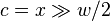
- i are low order bits,
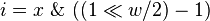
-
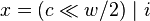
- conversion is in time

VEB recursive structure
- van Emde Boas structure (VEB) V of size u with word size w
- V consists of VEB structures of size and word size
 called clusters
- each cluster is denoted by V.cluster[c], for
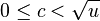
- if is contained in V and x is not the minimum, then i is contained in V.cluster[i]
- in addition, we maintain a summary VEB of size and word size , denoted by V.sumary
- summary contains all integers c such that V.cluster[c] is not empty
- we store minimum element of V separately in V.min (it is not in any cluster) or value None in case V is empty
- we also store copy of maximum element of V in V.max

Operations
Successor
- query for successor of in VEB V
- we first check if x is less then minimum of V, in that case minimum is the successor
- if x is less than maximum in it's own cluster, then the successor of x
must be in that cluster (it's either maximum of that cluster or some
other element), so we can recursively search for the successor in that
cluster
- otherwise, x is greater than any element in it's own cluster, so the answer is minimum in first non empty cluster that goes after cluster c, we can find it by recursive search in summary
- in each of three cases, we call recursion at most once on VEB of square root of size of V, so running time is bounded by recurrence

- predecessor query works in very similar fashion
Successor(V, x = <c,i>) {
    if (x < V.min) return V.min;
    if (i < V.cluster[c].max) {
        return <c, Successor(V.cluster[c], i)>;
    } else {
        c' = Successor(V.summary, c);
        return <c', V.cluster[c'].min>;
    }
}
Insert
- we want to insert into VEB V
- if minimum is None, it means V is empty and we just set minimum, maximum and return (since minimum is not stored recursively)
- if x is less than minimum, we swap values of x and minimum, so we will insert the old minimum
- if x is greater than maximum, we replace maximum with copy of x
- we check, whether cluster c is empty
- in case it is, we need to insert c into summary
- at last, we insert i into x's cluster c
- note that it can happen that we call recursion twice, but in that case cluster c was empty, so second insert (of i into cluster c) takes constant time, because it just sets minimum and returns
- in any case, we have at most one deep (and at most one shallow)
recursion, so running time is still bounded by aforementioned recurrence
Insert(V, x = <c,i>) {
    if (V.min == None) {
        V.min = V.max = x;
        return;
    }
    if (x < V.min) swap(x, V.min);
    if (x > V.max) V.max = x;
    if (V.cluster[c].min == None) {
        Insert(V.summary, c);
    }
    Insert(V.cluster[c], i);
}
Delete
- we want to remove from VEB V
- if x is minimum of V, we first check whether the summary is empty
- in case it is, x is the only element of V, so we just remove him and return
- in case there are more elements, new minimum is going to be minimum of first non-empty cluster (since x
is the overall minimum and is stored separately), which we can find
easily in constant time (we look at minimum of summary and take minimum
from that cluster)
- now, we need to delete either minimum of first non-empty cluster (because we moved it into V.min) or x (case where x is not minimum, so it is in some cluster)
- we delete our value recursively from it's cluster
- in case cluster we delete element from is now empty, we need to delete it's number from summary by second recursive call
- note that, same as with insert, in case of second recursive call,
cluster in first call had only one element, so it was shallow recursion
in constant time and we still have only one deep recursion
- finally, we set min and max values accordingly
Delete(V, x = <c,i>) {
    if (x == V.min) {
        c = V.summary.min
        if (c == None) {
            V.min = None;
            return;
        }
        V.min = <c, i = V.cluster[c].min>;
    }
    Delete(V.cluster[c], i);
    if (V.cluster[c].min == None) {
        Delete(V.summary, c);
    }
    if (V.summary.min == None) {
        V.max = V.min;
    } else {
        c' = V.summary.max;
        V.max = <c', V.cluster[c'].max>;
    }
}
Simple tree view
- original van Emde Boas data structure
- it is similar to previous structure, but from tree point of view
- take a bit vector v of size u, where i-th bit is 1, if integer i is in the structure and 0 otherwise
- next, build full binary tree over vector v, where at each node we store the OR of its children

- note that when we split tree in half of its height, first half represents summary (its leaves are summary bits) and size trees in second half represent clusters
- value of node in tree determine if there is some integer in interval that corresponds to that node
- we will also store for each tree node minimum and maximum integer that is in its interval
Predecessor, successor
- assume we are querying integer x and it is not in the set
- take path from x to root in tree and look at first 1 on that path
- let the last 0 be on node u and first 1 on node v
- if u is left child of v, it means the successor must be in right child's tree and it is minimum of that subtree (since value of v is 1, there must be element in right subtree of v)
- if u is right child of v, we can find predecessor of x as maximum from v's left subtree
- to compute successor from predecessor and vice versa, we can simply store all elements of the structure in sorted linked list
- to find 0-1 transition in x to root path, we use binary search on height
- as value of each node is OR of its children, every element to root
path is monotone, path starts as contiguous zeros followed by ones, so
we can binary search for 0-1 transition
- in RAM model, we can index directly into path, in other models
(e.g. pointer machine), we must store pointers to ancestors to quickly
jump in binary search
- in case x is in the set, we just use forward or backward pointer
- time complexity:
- as the binary tree has height w, cost of binary search is
 or
or 
Updates
- updating this structure is very expensive
- per operation, we must update all nodes of leaf-to-root path, in
 time
time
Sources
Perzistentné dátové štruktúry
Sources
Persistent data structures
- keep old versions of the data structure
- partial persistence: update only current version, query any old version, linearly ordered versions
- full persistence: update any version, versions form a tree
- confluent persistence: combine versions together, versions form a DAG
- fully functional: never modify nodes, only create new
- backtracking: query and update only current version, revert to an older version
- retroactive: insert updates to the past, delete past updates, query at any past time relative to current set of updates
Pointer machine
- model of computation, without arrays
- constant-size nodes, holding data (numbers, characters, etc) and pointers to other nodes
- pointers can be assigned: address of a newly created node, copy of another pointer, null
- no pointer arithmetic
- root node with all global variables, all variable names in the program of the form root.current.left.x
General transformation with node copying
First, let us prove that the algorithm for the update will terminate
- assume that outdegree of each node is at most 2p-1
- update on one node may trigger other updates etc, in the worst case the each newest node might be rebuilt (replaced by another)
- However, no node is replaced by a new node twice within one recursive update
- Assume by contradiction that such a node exists and consider the
first node that is rebuilt the second time. Between its first and second
rebuild it must have acquired 2p mods, but these mods must have been
caused by nodes to which this nodes points to being rebuilt. There are
at most 2p-1 such nodes and none of them was rebuilt more than once
because we consider the first node which is rebuilt twice.
Notes for the amortized analysis:
- as real cost, count the number of recursive calls (all other computation proportional to that)
- want to prove that the amortized cost of one update is 2
- if there is space in the node for another mod, real cost is 1 (only
one call to modify), change of potential is 1, so amortized cost is 2
- if the node is full, real cost is 1, change of potential is -2p
plus amortized cost of all subsequent recursive calls. By induction,
each of these calls has amortized cost 2, so overall amortized cost is 1
- what is the induction on? The depth in the tree of recursive calls
(leaves are the base cases where node not full). We have already proved
that this node is finite.
 zapíšeme ako <math>\sum_{k=0}^n k^2</math>.


![+,-,*,/,\%,\&,|,\gg ,\ll ,<,>,[~]](vpds-archiv_files/d826bb9c7483a8473ac4d0677a0d5974.png)


