Vybrané partie z dátových štruktúr
2-INF-237, LS 2016/17
Hešovanie
Obsah
Introduction to hashing
- Universe U = {0,..., u-1}
- Table of size m
- Hash function h : U -> {0,...,m-1}
- Let X be the set of elements currently in the hash table, n = |X|
- We will assume n = Theta(m)
Totally random hash function
- (a.k.a uniform hashing model)
- select hash value h(x) for each x in U uniformly independently
- not practical - storing this hash function requires u * lg m bits
- used for simplified analysis of hashing in ideal case
Universal family of hash functions
- some set of functions H
- draw a fuction h uniformly randomly from H
- there is a constant c such that for any distinct x,y from U we have Pr(h(x) = h(y)) <= c/m
- probability goes over choices of h
Note
- for totally random hash function, this probability is exactly 1/m
Example of a universal family:
- choose a fixed prime p >= u
- H_p = { h_a | h_a(x) =(ax mod p) mod m), 1<=a<=p-1 }
- p-1 hash functions, parameter a chosen randomly
Proof of universality
- consider x!=y, both from U
- if they collide (ax mod p) mod m = (ay mod p) mod m
- let c = (ax mod p), d = (ay mod p)
- note that c,d in {0..p-1}
- also c!=d because otherwise a(x-y) is divisible by p and both a and |x-y| are numbers from {1,...,p-1} and p is prime
- since c mod m = d mod m, then c-d = qm where 0<|qm|<p
- there are <=2(p-1)/m choices of q where |qm|<p
- we get a(x-y) mod p = qm mod p
- this has exactly one solution a in {1...p-1}
- if there were two solutions a1 and a2, then (a1-a2)(x-y) would be divisible by p, which is again not possible
- overall at most 2(p-1)/m choices of hash functions collide x and y
- out of p-1 all hash functions in H_p
- therefore probability of collision <=2/m
Hashing with chaining, using universal family of h.f.
- linked list (or vector) for each hash table slot
- let c_i be the length of chain i, let
 for x in U
- any element y from X s.t. x!=y maps to h(x) with probability <= c/m
- so E[C_x] <= 1 + n * c / m = O(1)
- from linearity of expectation - sum over indicator variables for each y in X if it collides with x
- +1 in case x is in X
- so expected time of any search, insert and delete is O(1)
- again, expectation taken over random choice of h from universal H
- however, what is the expected length of the longest chain in the table?
- O(1+ sqrt(n^2 / m)) = O(sqrt(n))
- see Brass, p. 382
- there is a matching lower bound
- for totally random hash function this is "only" O(log n / log log n)
- similar bound proved also for some more realistic families of hash functions
- so the worst-case query is on average close to logarithmic
References
- Textbook Brass 2008 Advanced data structures
- Lecture L10 Erik Demaine z MIT: http://courses.csail.mit.edu/6.851/spring12/lectures/
Perfect hashing
Static case
- Fredman, Komlos, Szemeredi 1984
- avoid any collisions, O(1) search in a static set
- two-level scheme: use a universal hash function to hash to a table of size m = Theta(n)
- each bucket i with set of elements X_i of size c_i hashed to a second-level hash of size m_i = alpha c_i^2 for some constant alpha
- again use a universal hash function for each second-level hash
- expected total number of collisions in a second level for slot i:
- sum_{x,y in X_i, x!=y} Pr(h(x) = h(y)) <= (c_i)^2 c/m_i = c/alpha = O(1)
- here c is the constant from definition universal family
- with a sufficently large alpha this expected number of collisions is <=1/2
- e.g. for c = 2 set alpha = 4
- then with probability >=1/2 no collisions by Markov inequality
- number of collisions is a random variable Y number with possible values 0,1,2,...
- if E[Y]<=1/2, Pr(Y>=1)<=1/2 and thus Pr(Y=0)>=1/2
- when building a hash table if we get a collision, randomly sample another hash function
- in O(1) expected trials get a good hash function
- expected space: m + sum_i m_i^2 = Theta(m + sum_i c_i^2)
- sum_i (c_i^2) is the number of pairs (x,y) s.t. x,y in X and h(x)=h(y); include x=y
-

- so expected space is linear
- can be made worst-case by repeating construction if memory too big
- expected construction time O(n)
Dynamic perfect hashing
- amortized vector-like tricks
- when a 2-nd level hash table gets too full, allocate a bigger one
- O(1) deterministic search
- O(1) amortized expectd update
- O(n) expected space
References
- Lecture L10 Erik Demaine z MIT: http://courses.csail.mit.edu/6.851/spring12/lectures/
- Textbook Brass 2008 Advanced data structures
Bloom Filter (Bloom 1970)
- supports insert x, test if x is in the set
- may give false positives, e.g. claim that x is in the set when it is not
- false negatives do not occur
Algorithm
- a bit string B[0,...,m-1] of length m, and k hash functions hi : U -> {0, ..., m-1}.
- insert(x): set bits B[h1(x)], ..., B[hk(x)] to 1.
- test if x in the set: compute h1(y), ..., hk(y) and check whether all these bits are 1
- if yes, claim x is in the set, but possibility of error
- if no, answer no, surely true
Bounding the error If hash functions are totally random and independent, the probability of error is approximately (1-exp(-nk/m))^k
- in fact probability somewhat higher for smaller values
- proof of the bound later
- totally random hash functions impractical (need to store hash value for each element of the universe), but the assumption simplifies analysis
- if we set k = ln(2) m/n, get error
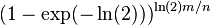 .
.
-
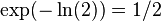 and thus we get error
 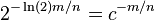 , where
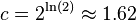
- to get error rate p for some n, we need

- for 1% error, we need about m=10n bits of space and k=7
- memory size and error rate are independent of the size of the universe U
- compare to a hash table, which needs at least to store data items themselves (e.g. in n lg u bits)
- if we used k=1 (Bloom filter with one hash function), we need m=n/ln(1/(1-p)) bits, which for p=0.01 is about 99.5n, about 10 times more than with 7 hash functions
Use of Bloom filters
- e.g. an approximate index of a larger data structure on a disk - if x not in the filter, do not bother looking at the disk, but small number of false positives not a problem
- Example: Google BigTable maps row label, column label and timestamp to a record, underlies many Google technologies. It uses Bloom filter to check if a combination of row and column label occur in a given fragment of the table
- For details, see Chang, Fay, et al. "Bigtable: A distributed storage system for structured data." ACM Transactions on Computer Systems (TOCS) 26.2 (2008): 4. [1]
- see also A. Z. Broder and M. Mitzenmacher. Network applications of Bloom filters: A survey. In Internet Math. Volume 1, Number 4 (2003), 485-509. [2]
Proof of the bound
- probability that some B[i] is set to 1 by hj(x) is 1/m
- probability that B[i] is not set to 1 is therefore 1-1/m and since we use k independent hash functions, the probability that B[i] is not set to one by any of them is (1-1/m)^k
- if we insert n elements, each is hashed by each function independently of other elements (hash functions are random) and thus Pr(B[i]=0)=(1-1/m)^{nk}
- Pr(B[i]=1) = 1-Pr(B[i]=0)
- consider a new element y which is not in the set
- error occurs when B[hj(y)]==1 for all j=1..k
- assume for now that these events are independent for different j
- error then occurs with probability Pr(B[i]=1)^k = (1-(1-1/m)^{nk})^k
- recall that
- thus probability of error is approximately (1-exp(-nk/m))^k
However, Pr(B[i]=1) are not independent
- consider the following experiment: have 2 binary random variables Y1, Y2, each generated independently, uniformly (i.e. P(Y1=1) = 0.5)
- Let X1 = Ya and X2 = Yb where a and b are chosen independently uniformly from set {1,2}
- X1 and X2 are not independent, e.g. Pr(X2 = 1|X1 = 1) = 2/3, whereas Pr(X2=1) = 1/2. (check the constants!)
- note: X1 and X2 would be independent conditioned on the sum of Y1+Y2.
- In Mitzenmacher & Upfal (2005), pp. 109–111, 308. - less strict independence assumption
Exercise Let us assume that we have separate Bloom filters for sets A and B with the same set k hash functions. How can we create Bloom filters for union and intersection? Will the result be different from filter created directly for the union or for the intersection?
Theory
- Bloom filter above use about 1.44 n lg(1/p) bits to achieve error rate p. There is lower bound of n lg(1/p) [Carter et al 1978], constant 1.44 can be improved to 1+o(1) using more complex data structures, which are then probably less practical
- Pagh, Anna, Rasmus Pagh, and S. Srinivasa Rao. "An optimal Bloom filter replacement." SODA 2005. [3]
- L. Carter, R. Floyd, J. Gill, G. Markowsky, and M. Wegman. Exact and approximate membership testers. STOC 1978, pages 59–65. [4]
- see also proof of lower bound in Broder and Mitzenmacher 2003 below
Counting Bloom filters
- support insert and delete
- each B[i] is a counter with b bits
- insert increases counters, delete decreases
- assume no overflows, or reserve largest value 2^b-1 as infinity, cannot be increased or decreased
- Fan, Li, et al. "Summary cache: A scalable wide-area web cache sharing protocol." ACM SIGCOMM Computer Communication Review. Vol. 28. No. 4. ACM, 1998. [5]
References
- Bloom, Burton H. (1970), "Space/Time Trade-offs in Hash Coding with Allowable Errors", Communications of the ACM 13 (7): 422–426
- Bloom filter. In Wikipedia, The Free Encyclopedia. Retrieved January 17, 2015, from http://en.wikipedia.org/w/index.php?title=Bloom_filter&oldid=641921171
- A. Z. Broder and M. Mitzenmacher. Network applications of Bloom filters: A survey. In Internet Math. Volume 1, Number 4 (2003), 485-509. [6]
Locality Sensitive Hashing
- todo: expand and according to slides
- typical hashing tables used for exact search: is x in set X?
- nearest neighbor(x): find y in set X minimizing d(x,y) for a given distance measure d
- or given x and distance threshold r, find all y in X with d(x,y)<=r
- want: polynomial time preprocessing of X, polylogarithmic queries
- later in the course: geometric data structures for similar problems in R^2 or higher dimensions
- but time or space grows exponentially with dimension (alternative is linear search) - "curse of dimensionality"
- examples of high-dimensional objects: images, documents, etc.
- locality sensitive hashing (LHS) is a randomized data structure not guaranteed to find the best answer but better running time
Approximate near neighbour (r,c)-NN
- preprocess a set X of size n for given r,c
- query(x):
- if there is y in X such that d(y,x)<=r, return z in X such that d(z,x)<=c*r
- LHS returns such z with some probability at least f
Example for Hamming distance in binary strings of length d
- Hash each string using L hashing functions, each using O(log n) randomly chosen string positions (hidden constant depends on d, r, c), then rehash using some other hash function to tables of size O(n) or a single table of size O(nL)
- Given q, find it using all L hash function, check every collision, report if distance at most cr. If checked more than 3L collisions, stop.
- L = O(n^{1/c})
- Space O(nL + nd), query time O(Ld+L(d/r)log n)
- Probability of failure less than some constant f < 1, can be boosted by repeating independently
Minimum hashing
- similarity of two sets measured as Jaccard index J(A,B) = |A intersect B | / | A union B |
- distance d(A,B) = 1-J(A,B)
- used e.g. for approximate duplicate document detection based on set of words occurring in the document
- choose a totally random hash function h
- minhash_h(A) = \min_{x\in A} h(x)
- Pr(minhash_h(A)=minhash_h(B)) = J(A,B) = 1-d(A,B) if using totally random hash function an no collisions in A union B
- where can be minimum in union? if in intersection, we get equality, otherwise not
- (r_1, r_2, 1-r_1, 1-r_2)-sensitive family (if we assume no collisions)
- again can we apply amplification
Notes
- Real-valued vectors: map to bits using random projections sgn (w · x + b)
- Data-dependent hashing: Use PCA, optimization, kernel tricks, even neural networks to learn hash functions good for a particular set of points and distance measure (or learn even distance measure from examples). [7]
Sources
- Har-Peled, Sariel, Piotr Indyk, and Rajeev Motwani. "Approximate Nearest Neighbor: Towards Removing the Curse of Dimensionality." Theory of Computing 8.1 (2012): 321-350. [8]
- Indyk and Motwani: Approximate nearest neighbors: Towards removing the curse of dimensionality. In Proc. 30th STOC, pp. 604–613. ACM Press, 1998.
- http://www.mit.edu/~andoni/LSH/ Pointers to papers
- Wikipedia
- Several lectures:
- http://infolab.stanford.edu/~ullman/mining/2009/similarity3.pdf various distances, connection to minhashing
- https://users.soe.ucsc.edu/~niejiazhong/slides/kumar.pdf nic intro, more duplicate detection, NN at the end
- http://delab.csd.auth.gr/courses/c_mmdb/mmdb-2011-2012-lsh2.pdf also nice intro through Hamming
- Charikar, Moses S. "Similarity estimation techniques from rounding algorithms." STOC 2002 [9]
- simHash (cosine measure)